Total Mechanical Energy Conservation – Escape Velocity & Binding Energy – Einstein Field Equation

The study of Euclidean Spherical Mechanics, is a set of conceptual and mathematical tools, used to describe the physics of a spherically symmetric system mass body that creates its own gravitational field, while; at rest/static, in relativistic motion, spinning/rotating at rest, or spinning/rotating while in motion.
The Euclidean Spherical Mechanics takes into account the relativity of different measuring observers, and different frames of reference; a “proper observer” located at the center of the sphere, and an “external observer” located at the surface of the sphere.
The Euclidean Spherical Mechanics unifies and generalizes, the theories, concepts, and mathematics of “Special Theory of Relativity” and “General Theory of Relativity” into a single framework known as the “Super Special Theory of Relativity”.
Under the condition where, only conservative forces do work, the “Total Mechanical Energy” of an isolated “Net Inertial Mass” system body remains “constant” and “conservative”. The “Total Mechanical Energy” of an isolated system is constant, means that any increase in “Kinetic Energy” is always accompanied by a decrease in the “Potential Energy” of the system.
This fundamental principle of the conservation of energy, of the “Total Mechanical Energy”, of any isolated and adiabatic system, is one of the most fundamental and important concepts of physics; which is why I am writing a second article on the subject.
The conservation of energy is also stated conceptually: Energy is never created or destroyed in the system; but energy changes from one form, into another form. For example, mechanical energy can be transformed into electrical energy, which can be further transformed into chemical energy.
In this work, a practical application of the Total Mechanical Energy is discussed; which includes a generalization of the Einstein Field Equation – Total Mechanical Energy.
In this work only the “Total Mechanical Energy” and that being the net sum of the “Net Kinetic Energy” ( ), and the “Gravitational Potential Energy” (
 ) associated with the “Gravitational Force” (
 ) of the system mass body is considered.
Total Mechanical Energy


Now, consider that a “test mass” object is located in a gradient gravitational field, and is projected out from a “lower gravitational potential” of the gradient, into a “higher gravitational potential” in the field; with a certain “Kinetic Energy” ().
The “test mass” object has an initial “Kinetic Energy” () and an initial “Speed”, as it moves up the gradient escaping the field, with decreasing speed, until the increase in the “Potential Energy” (), equals to the value of a decrease in the “Kinetic Energy” (), of the conserved system.
The “test mass” object, then stops and falls back towards the center of the gradient field, losing potential energy, and gaining in kinetic energy. At an infinite distance from the center of the gradient gravity potential, the “Potential Energy” ( ) is equal to zero (0).
When the “test mass” object is located at a specific potential in the gradient gravitational field with a negative “Potential Energy” ( ), this is considered the “strongly bound” to the potential, energy condition; and is the greatest possible decrease in the energy of the conserved system.
The “Escape Energy” in this case, would be the greatest possible increase that the “test mass” can achieve, moving in an opposite direction through the gradient field, and is given by the positive value of the, “Potential Energy” ( ), which is equal and opposite, to the value of the negative potential energy, “strongly bound” condition.
The greatest possible increase in “Potential Energy” (), equals to the greatest possible decrease in the “Kinetic Energy” (). If the “test mass” has an initial “Kinetic Energy” ( ), that is greater than the negative of the “Potential Energy” (
 ), the “test mass” object will never stop and fall towards lower gravity gradient potentials, but “Escapes” into outer space.
Now, let’s consider “Ionization” of the “Hydrogen Atom”, and the, “Gravitational Vortex” model in the “Ground State”. The electron exists in a spherical volume, surrounding a smaller spherical volume of the proton; A simple “Hydrogen Atom” is comprised of one electron unit, and one proton unit. The electron existing in a spherical volume spins and takes (720) degrees to make a return to its initial starting point; which is considered a complete rotation; and is not the familiar (360) degrees. This is also called the “Spin 1/2” quantum state.
The familiar (360) degrees complete rotation of the the two spin state system, is folded in, and is described on spherical surface, and is output or result, in the form of the Geodesic Arc-Length – Map/Patch/Manifold Angle ( ).
).
This means that the electon must have two spin states. The electron in spherical volume about the proton is described by two independent rotations; one spin rotation in the “latitude” ( ) direction, and another spin rotation of the sphere, in the “longitude” (
 ) direction; and is described by the Geodesic Arc-Length – Map/Patch/Manifold Angle (
 ) Metric on the surface of an electron spheroid, given by the following.
![{\Omega^2_{Map}}_{(\theta \phi)}\;=\;(-)(\frac{\vec{c^2_{Light}}}{r^2})\,{\Delta{t^2_{Map}}}\;=\;[\vec{\theta^2_{Lat}}\,\,+\,\,\sin^2\theta_{Lat}\,\vec{\phi^2_{Lon}}]](https://s0.wp.com/latex.php?latex=%7B%5COmega%5E2_%7BMap%7D%7D_%7B%28%5Ctheta+%5Cphi%29%7D%5C%3B%3D%5C%3B%28-%29%28%5Cfrac%7B%5Cvec%7Bc%5E2_%7BLight%7D%7D%7D%7Br%5E2%7D%29%5C%2C%7B%5CDelta%7Bt%5E2_%7BMap%7D%7D%7D%5C%3B%3D%5C%3B%5B%5Cvec%7B%5Ctheta%5E2_%7BLat%7D%7D%5C%2C%5C%2C%2B%5C%2C%5C%2C%5Csin%5E2%5Ctheta_%7BLat%7D%5C%2C%5Cvec%7B%5Cphi%5E2_%7BLon%7D%7D%5D&bg=ffffff&fg=333333&s=1&c=20201002)
![{\Omega^2_{Map}}_{(\theta \phi)}\;\;=\;\;{\omega^2_{\Omega}}\,{\Delta{t^2_{Light}}}\;\;=\;[{\omega^2_{\theta}\;+\;(sin^2\theta_{Lat})\,\omega^2_{\phi}}]\,{\Delta{t^2_{Light}}}](https://s0.wp.com/latex.php?latex=%7B%5COmega%5E2_%7BMap%7D%7D_%7B%28%5Ctheta+%5Cphi%29%7D%5C%3B%5C%3B%3D%5C%3B%5C%3B%7B%5Comega%5E2_%7B%5COmega%7D%7D%5C%2C%7B%5CDelta%7Bt%5E2_%7BLight%7D%7D%7D%5C%3B%5C%3B%3D%5C%3B%5B%7B%5Comega%5E2_%7B%5Ctheta%7D%5C%3B%2B%5C%3B%28sin%5E2%5Ctheta_%7BLat%7D%29%5C%2C%5Comega%5E2_%7B%5Cphi%7D%7D%5D%5C%2C%7B%5CDelta%7Bt%5E2_%7BLight%7D%7D%7D&bg=ffffff&fg=333333&s=1&c=20201002)
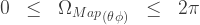
The Geodesic Arc-Length – Map/Patch/Manifold Angle (), can be used to derive an equation for the total “spin states” on the surface of an electron spheroid; resulting in the following range of values for rotation.

In the lowest spherical potential of the “Hydrogen Atom”, the “Ground State”, the radius of the orbit, potential, or volume, equals the “Bohr Radius” ( ) of the atom.
The various energy states (cases or conditions) that exists along a “Potential Energy” curve, for the “electron” and “proton” atomic system, has the same form, as that for a “satellite” orbiting the “earth”.
The “Electrostatic Potential Energy” ( ) of the “Hydrogen Atom”, two-body interacting system is described similarily to the “Gravitational Potential Energy” (
 ), being the energy of an infinite number of concentric spherical shells of gradient potentials of energy.
For the “Hydrogen Atom” system mass body, the “Ground State” potential, is the “energy state”, of the greatest quantity of attraction energy of system; and is considered to be a “Bound Strongly” to an “Electrostatic Potential” energy field condition; described by the following equation.


Because the “electron” is considered to be orbiting the “proton” in an “Electrostatic Potential”; the magnitude of the “Total Mechanical Energy” of the “electron” in the “Orbiting Energy” condition of the “Hydrogen Atom” system, must therefore, equal to the “Kinetic Energy”; which must equal to the one half of the magnitude of the “Potential Energy”.
This means that electrons, protons, and hydrogen atoms, similar to planets, moons, and solar systems, due to their, mass and energy, “warp”, space and time, in their local vicinities, producing curvature in the physical form of, a gradient field of “Potential Energy Potentials”, and a gradient field of “Kinetic Energy Potentials”.
The minimum additional energy a “satellite” orbiting the “earth”, or an “electron” orbiting the “proton”, must be given to “Escape” from the “earth”, or to “Escape” the “proton”, is the “Escape Energy” condition. The “Kinetic Energy” of the orbiting electron or satellite in a fixed potential, must therefore be doubled during the “Escape Energy” condition; given by the following equations.
Gravitational System – Escape Energy – Earth & Satellite – Circular Orbit


************************************************************
Gravitational System – Escape Energy – Proton & Electron – Circular Orbit

************************************************************
Electrostatic System – Escape Energy – Proton & Electron – Circular Orbit


This result of the “Escape Energy” condition, is that the “Kinetic Energy” is one half (1/2) the magnitude of the “Potential Energy” holds for any “Orbiting” condition, where the “Central Force” of attraction, that being the Gravitational Force ( ) or the Electrostatics Force (
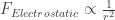 ); is inversely proportional to the square of the distance, relative to the center of any gradient field, of energy potentials.
The “Total Mechanical Energy” of the “electron” in “Orbit Condition” about the proton in the Hydrogen Atom, system is given by the following.


************************************************************

The approximate value of the “Total Mechanical Energy” in “Ground State” of the “Hydrogen Atom” two-body system, is given by the following.

In order to “ionize”, remove, or liberate the electron from the “Ground State” electrostatic energy potential, of the “Hydrogen” atomic system; the atom, must be given an “additional” amount of “supplied energy”, this surplus in energy is called the “Binding Energy” ( ), of the atom.
Thus, the energy required to remove or liberate the electron from the atom, is called “ionization”; and the “Binding Energy” is also called the “Ionization Energy”.
************************************************************
The Electrostatic Field – Total Mechanical Energy – “Orbiting” in gradient field, of energy potential, condition:

The Electrostatic Field – Total Mechanical Energy – “Escaping” from gradient field, of energy potential, condition:

************************************************************

************************************************************
(1) The Total Mechanical Energy Conservation – Euclidean Spherical Mechanics
Now that all of the physics terms and basic concepts have been discussed, let’s complete the conceptual and mathematical discussion of the Total Mechanical Energy Conservation ( ) in a consideration for various “Bound Potential Energy” and “Escape Potential Energy” conditional cases, and in consideration for “The General Theory of Relativity”.
The “math” and “physics” that will be discussed in the next few sections, are employed from work, that was derived in the articles below:
A Theory of Gravity for the 21st Century – The Gravitational Force and Potential Energy – in consideration with Special Relativity & General Relativity
Euclidean Spherical Mechanics – Total Mechanical Energy Conservation – in consideration with General Relativity
************************************************************
Total Mechanical Energy Conservation


Next substituting the appropriate “Kinetic Energy” and “Gravitational Potential Energy” terms yields:
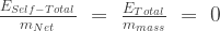
![\frac{E_{Self-Total}}{m_{Net}}\,\,=\,\,\frac{E_{Total}}{m_{mass}}\,\,=\,\,[\frac{1}{2}{|\vec{v}|^2_{CM}}\;\;-\;\;\frac{m_{Net}\,G}{r}]](https://s0.wp.com/latex.php?latex=%5Cfrac%7BE_%7BSelf-Total%7D%7D%7Bm_%7BNet%7D%7D%5C%2C%5C%2C%3D%5C%2C%5C%2C%5Cfrac%7BE_%7BTotal%7D%7D%7Bm_%7Bmass%7D%7D%5C%2C%5C%2C%3D%5C%2C%5C%2C%5B%5Cfrac%7B1%7D%7B2%7D%7B%7C%5Cvec%7Bv%7D%7C%5E2_%7BCM%7D%7D%5C%3B%5C%3B-%5C%3B%5C%3B%5Cfrac%7Bm_%7BNet%7D%5C%2CG%7D%7Br%7D%5D&bg=ffffff&fg=333333&s=1&c=20201002)
![\frac{E_{Self-Total}}{m_{Net}}\,\,=\,\,\frac{E_{Total}}{m_{mass}}\,\,=\,\,[\frac{1}{2}{|\vec{v}|^2_{CM}}\,\,-\,\,{g_{Gravity}}\,{r}]](https://s0.wp.com/latex.php?latex=%5Cfrac%7BE_%7BSelf-Total%7D%7D%7Bm_%7BNet%7D%7D%5C%2C%5C%2C%3D%5C%2C%5C%2C%5Cfrac%7BE_%7BTotal%7D%7D%7Bm_%7Bmass%7D%7D%5C%2C%5C%2C%3D%5C%2C%5C%2C%5B%5Cfrac%7B1%7D%7B2%7D%7B%7C%5Cvec%7Bv%7D%7C%5E2_%7BCM%7D%7D%5C%2C%5C%2C-%5C%2C%5C%2C%7Bg_%7BGravity%7D%7D%5C%2C%7Br%7D%5D&bg=ffffff&fg=333333&s=1&c=20201002)
![\frac{E_{Self-Total}}{m_{Net}}\,\,=\,\,\frac{E_{Total}}{m_{mass}}\,\,=\,\,\,[\frac{1}{2}{|\vec{v}|^2_{CM}}\,\,-\,\,{v^2_{Gravity}}]](https://s0.wp.com/latex.php?latex=%5Cfrac%7BE_%7BSelf-Total%7D%7D%7Bm_%7BNet%7D%7D%5C%2C%5C%2C%3D%5C%2C%5C%2C%5Cfrac%7BE_%7BTotal%7D%7D%7Bm_%7Bmass%7D%7D%5C%2C%5C%2C%3D%5C%2C%5C%2C%5C%2C%5B%5Cfrac%7B1%7D%7B2%7D%7B%7C%5Cvec%7Bv%7D%7C%5E2_%7BCM%7D%7D%5C%2C%5C%2C-%5C%2C%5C%2C%7Bv%5E2_%7BGravity%7D%7D%5D&bg=ffffff&fg=333333&s=1&c=20201002)
************************************************************
The Total Mechanical Energy Conservation described in “Classical Newtonian Mechanics” “ordinary” mathematical form.
![\frac{E_{Total}}{m_{Mass}}\,\,=\,\,\frac{1}{m_{Mass}}[{T_{Kinetic-Energy}}\;\;+\;\;{V_{Gravity-Potential}}]](https://s0.wp.com/latex.php?latex=%5Cfrac%7BE_%7BTotal%7D%7D%7Bm_%7BMass%7D%7D%5C%2C%5C%2C%3D%5C%2C%5C%2C%5Cfrac%7B1%7D%7Bm_%7BMass%7D%7D%5B%7BT_%7BKinetic-Energy%7D%7D%5C%3B%5C%3B%2B%5C%3B%5C%3B%7BV_%7BGravity-Potential%7D%7D%5D&bg=ffffff&fg=333333&s=1&c=20201002)
************************************************************
The Total Mechanical Energy Conservation described in “Spherical Euclidean Mechanics & General Relativity” “ordinary” mathematical form; and as a function of the Gradient Gravitational Field Inertial Potential (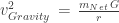 ), and the Speed of Light Inertia Potential (
 ).
).
![\frac{E_{Total}}{m_{mass}}\,\,=\,\,[\frac{1}{2}\,{c^2_{Light}}\,[\frac{({\Omega_{Map}}_{(\theta \phi)})^2}{2\,(ln(\frac{{c^2_{Light}}}{2\,{v^2_{Gravity}}}))^2\,\,+\,\,({\Omega_{Map}}_{(\theta \phi)})^2}]^2\,\,\,-\,\,\,{v^2_{Gravity}}]](https://s0.wp.com/latex.php?latex=%5Cfrac%7BE_%7BTotal%7D%7D%7Bm_%7Bmass%7D%7D%5C%2C%5C%2C%3D%5C%2C%5C%2C%5B%5Cfrac%7B1%7D%7B2%7D%5C%2C%7Bc%5E2_%7BLight%7D%7D%5C%2C%5B%5Cfrac%7B%28%7B%5COmega_%7BMap%7D%7D_%7B%28%5Ctheta+%5Cphi%29%7D%29%5E2%7D%7B2%5C%2C%28ln%28%5Cfrac%7B%7Bc%5E2_%7BLight%7D%7D%7D%7B2%5C%2C%7Bv%5E2_%7BGravity%7D%7D%7D%29%29%5E2%5C%2C%5C%2C%2B%5C%2C%5C%2C%28%7B%5COmega_%7BMap%7D%7D_%7B%28%5Ctheta+%5Cphi%29%7D%29%5E2%7D%5D%5E2%5C%2C%5C%2C%5C%2C-%5C%2C%5C%2C%5C%2C%7Bv%5E2_%7BGravity%7D%7D%5D&bg=ffffff&fg=333333&s=1&c=20201002)
************************************************************
The Total Mechanical Energy Conservation described in “Spherical Euclidean Mechanics & General Relativity” “ordinary” mathematical form; and as a function of the Semi-Major Radius ( ) which is measured from the center of the field and relative to the Schwarzschild Radius (
 ) Black Hole Event Horizon.
![\frac{E_{Total}}{m_{mass}}\,\,=\,\,[\frac{m_{Net}\,G}{r_{Schwarzschild}}\,[\frac{({\Omega_{Map}}_{(\theta \phi)})^2}{2\,(ln(\frac{r}{r_{Schwarzschild}}))^2\,\,+\,\,({\Omega_{Map}}_{(\theta \phi)})^2}]^2\,\,-\,\,\frac{m_{Net}\,G}{r}]](https://s0.wp.com/latex.php?latex=%5Cfrac%7BE_%7BTotal%7D%7D%7Bm_%7Bmass%7D%7D%5C%2C%5C%2C%3D%5C%2C%5C%2C%5B%5Cfrac%7Bm_%7BNet%7D%5C%2CG%7D%7Br_%7BSchwarzschild%7D%7D%5C%2C%5B%5Cfrac%7B%28%7B%5COmega_%7BMap%7D%7D_%7B%28%5Ctheta+%5Cphi%29%7D%29%5E2%7D%7B2%5C%2C%28ln%28%5Cfrac%7Br%7D%7Br_%7BSchwarzschild%7D%7D%29%29%5E2%5C%2C%5C%2C%2B%5C%2C%5C%2C%28%7B%5COmega_%7BMap%7D%7D_%7B%28%5Ctheta+%5Cphi%29%7D%29%5E2%7D%5D%5E2%5C%2C%5C%2C-%5C%2C%5C%2C%5Cfrac%7Bm_%7BNet%7D%5C%2CG%7D%7Br%7D%5D&bg=ffffff&fg=333333&s=1&c=20201002)
************************************************************
The Total Mechanical Energy Conservation described in “Spherical Euclidean Mechanics & General Relativity” “ordinary” mathematical form; and as a function of the Linear Mass Density ( ) which is measured from the center of the field and relative to the Black Hole Linear Mass Density (
 ) constant.
![\frac{E_{Total}}{m_{mass}}\,\,=\,\,[{\mu_{L-Density}}_{BH}\,G\,[\frac{({\Omega_{Map}}_{(\theta \phi)})^2}{2\,(ln(\frac{{\mu_{L-Density}}_{BH}}{{\mu_{L-Density}}}))^2\,\,+\,\,({\Omega_{Map}}_{(\theta \phi)})^2}]^2\,\,-\,\,{\mu_{L-Density}}\,G]](https://s0.wp.com/latex.php?latex=%5Cfrac%7BE_%7BTotal%7D%7D%7Bm_%7Bmass%7D%7D%5C%2C%5C%2C%3D%5C%2C%5C%2C%5B%7B%5Cmu_%7BL-Density%7D%7D_%7BBH%7D%5C%2CG%5C%2C%5B%5Cfrac%7B%28%7B%5COmega_%7BMap%7D%7D_%7B%28%5Ctheta+%5Cphi%29%7D%29%5E2%7D%7B2%5C%2C%28ln%28%5Cfrac%7B%7B%5Cmu_%7BL-Density%7D%7D_%7BBH%7D%7D%7B%7B%5Cmu_%7BL-Density%7D%7D%7D%29%29%5E2%5C%2C%5C%2C%2B%5C%2C%5C%2C%28%7B%5COmega_%7BMap%7D%7D_%7B%28%5Ctheta+%5Cphi%29%7D%29%5E2%7D%5D%5E2%5C%2C%5C%2C-%5C%2C%5C%2C%7B%5Cmu_%7BL-Density%7D%7D%5C%2CG%5D&bg=ffffff&fg=333333&s=1&c=20201002)
************************************************************
Black Hole Linear Mass Density

************************************************************
Where the Geodesic Arc-Length – Map/Patch/Manifold Angle () Metric on the surface of a spheroid is given by the following.
![{\Omega^2_{Map}}_{(\theta \phi)}\;\;=\;\;[\vec{\theta^2_{Lat}}\;\;+\;\;\sin^2\theta_{Lat}\,\vec{\phi^2_{Lon}}]](https://s0.wp.com/latex.php?latex=%7B%5COmega%5E2_%7BMap%7D%7D_%7B%28%5Ctheta+%5Cphi%29%7D%5C%3B%5C%3B%3D%5C%3B%5C%3B%5B%5Cvec%7B%5Ctheta%5E2_%7BLat%7D%7D%5C%3B%5C%3B%2B%5C%3B%5C%3B%5Csin%5E2%5Ctheta_%7BLat%7D%5C%2C%5Cvec%7B%5Cphi%5E2_%7BLon%7D%7D%5D&bg=ffffff&fg=333333&s=1&c=20201002)
************************************************************
(2) The Net Kinetic Energy in direct relation to the – Stress Energy of the Einstein Field Equation
The General Relativity – Einstein Field Equation determines the metric of a “gravity vortex” in the “Vacuum of Space-time” for a given arrangement of “Stress-Energy” ( ) in any localized region of space and time, and where matter and energy is condensed and localized, space and time there is warped, bent, or curved.
The General Relativity – Einstein Field Equation declares that the attractive force of gravity, is communicated in time, to any unit of matter, located within a gradient gravitational field, at the “Speed of Light”. This is in contradiction with Isaac Newton’s concept of the attractive force of gravity, in which he theorized, that gravity was being communicated to any unit of matter, located within a gradient gravitational field, “Instantaneously”.
The General Relativity – Einstein Field Equation also declares that the attractive “Gravitational Force” that mass, exerts on other mass objects, located at some distance away from their respective centers, is due to the curvature of the “Vacuum of Space-time”. The attractive Gravitational Force is therefore, the result of the masses and their energies, warping and curving, space, and time in their respective vicinities.
All mass or matter, curves space and time in its local vicinity, in the form of a field of gradient energy potentials. The mass includes the mass of the electron, the mass of the proton, the mass of the hydrogen atom, the mass of a molecule, the mass of the earth, the mass of the moon, the mass of the sun, and the mass of the galaxy; all warp and curve, space, and time in their respective vicinities.
Thus, the masses immersed in the gradient gravitational field vortex, will follow a geodesic or curved path, created by the presence of mass and energy warping and curving the “Vacuum of Space-time” in the local vicinity of mass and energy.

The General Relativity – Einstein Field Equation also predicts that the “Vacuum of Spacetime”, also is known as the “Universal Vacuum Energy”, is an elastic continuum, from which a “gravity vortex” of gradient energy potentials evolves; and is measured by the localized evolution and condensing of the “Stress ‘Kinetic ‘Energy” of the universal vacuum energy, into matter, or mass units.
The “Stress ‘Kinetic ‘Energy” is a measure of an elastic energy of the universal vacuum, that changes in direct proportion to the distance, and time, or space-time, as measured from the center of the gradient gravity field; and likewise is directly proportional to the “Net Inertial Mass” ( ) of the gradient gravitational field.
The “Stress Energy” of the “Einstein Field Equation” in “General Relativity” measures the elasticity of space and time surrounding a system mass body, and manifest in the form of an infinite series of concentric spherical shells, which, warp, deform, and curve, space and time, in the local vicinity of the “Net Inertial Mass” (), as spherical gradient grid; and is described by a linear relationship between the “Stress Pressure” which is pressure acting normal to a spheroid surface and the “Strain Pressure” which is pressure acting tangential to a spheroid surface.

The “Stress Energy” () of the Einstein Field Equation is actually a measure of the “Kinetic Energy” and not the “Potential Energy” of an isolated system mass body. The “Stress Energy” () of the Einstein Field Equation is a measure of infinite number of concentric spherical gradient gravitational field of “Kinetic Energy Potentials”.
The “Kinetic Energy Potentials” of a gradient gravitational field, are not the same as the gradient gravitational field “Potential Energy Potentials”; although both field potentials exists at the same location in space, relative to the center of the gradient field.
The General Relativity – Einstein Field Equation predicts that since the “Vacuum of Spacetime”, is an elastic continuum, from which evolves a “Gravity Vortex” of matter, and is measured by the localized condensing of the “Stress Energy” () of the universal vacuum into units of “mass”.
The “Stress ‘Kinetic ‘Energy” ( ) of the universal vacuum changes in direct proportion to the distance and time (space-time), and produces a constant; such that there is a “Cosmic ‘Dark’ Vacuum Force” (
 ) that is a constant of Nature.


************************************************************
Where the “Energy Source” and “Distance” of “Minimum Curvature” is described by the following Einstein, universal “vacuum force” constant ratio;

And the “Energy Field” and “Distance” of “Maximum Curvature” is described by the following Ricci/Riemannian, universal “vacuum force” constant ratio;

************************************************************
“Vacuum Energy” and “Vacuum Force” is an underlying background energy that permeates all of mass, space, and time in the universe. The “vacuum energy” on a fundamental level is the substratum substance of matter, space, time. Therfore, the “vacuum” in nature is, not empty at all, but is seething with energy, even when devoid of inertial matter. This means that the concept of “vacuum” must be described with the physics, such that it supports both Baryonic Matter, and Non Baryonic Matter. The Non Baryonic Matter is thus, the fundamental energy of the vacuum!
The Vacuum energy of the universe which shall be synonymous with the Aether, is a gas comprised of discrete units and according to ancient and medieval science, the Aether also spelled æther or ether, is the material that fills all regions of the Universe!
The “Vacuum Force” is the cause of the constant flow of a ‘Aether” fluid into a partial vacuum, or region of low pressure. The pressure gradient between this region and the ambient pressure will propel matter toward the low pressure area.
The Vacuum “Dark” Cosmic Force of Spacetime () is a “universal constant” force of interaction upon matter, and is pervasive throughout the universe, and acts on all mass bodies at all times; and is invariant to all frames of reference, and is independent of any changes in mass, space, or time.
The Vacuum “Dark” Cosmic Force of Spacetime () is the “constant” force of the universal continuum, the “Vacuum of Space-time”. The Vacuum “Dark” Cosmic Force of Spacetime () is the force of interaction upon matter, and represents where matter, energy, space, and time, are intertwined in the substratum of the vacuum; the elastic energy of the universe.
Definition:
The strength of the Cosmic “Dark” Vacuum Force () is a universal constant force that acts on all bodies immersed in the universe, at all times; and is equal to the square of the Aether Gravitation Light Force ( ) divided by four (4) times the Inertial Mass Gravitational Self Force (
 ); and likewise is equal to one fourth, the fourth power of the Speed of Light (
 ) divided by the Universal Gravitational Constant (G).
Cosmic “Dark” Vacuum Force


************************************************************
Cosmic “Dark” Vacuum Force – constant


************************************************************
Where the Aether Gravitational Light Force ( ) is given by the following.

************************************************************
Where the Inertial Mass Gravitational Self Force ( ) is given by the following.

************************************************************
The “Stress Energy” () of the Einstein Field Equation
The “Stress” Kinetic Energy () measures “Kinetic Energy Potentials of a gradient gravity field, and describes the “gravitational vortex” energy of curved space-time gravity potentials, in the presence matter and energy; which includes both energy and momentum densities, as well as stress pressure, and shear pressure.
Drawing further upon the analogy with Newtonian gravity, it is natural to assume that the field equation for gravity describes this “Stress” Kinetic Energy (), on the surface of a spherical gravitational field of “Kinetic Energy Potentials”; which can be considered states in an Ideal Gas Equation of State of the “Vacuum of Space-time”.
The Vacuum of Spacetime is an elastic energy, from which a “gravity vortex” evolves, of concentric spherical shells of energy potentials; which can be considered “gas energy states”. These “gas energy states” are also described by an “Ideal Gas Equation of State”, where the gas “Pressure” ( ), “Volume” (
 ), and gas “Temperature” (
 ), are all conjugate of one another.
Ideal Gas Equation for Vacuum of Spacetime – Kinetic Stress Energy


Where, the symbol (N) denotes the total number of constituents, of the “Gravitational Vortex” system body.
And, the Boltzmann Constant is given by

************************************************************
Vacuum of Spacetime – Einstein Field Equation – “Space & Time” Stress Energy
The “Stress Energy” ( ) changes linearly with increasing gradient field “distance” (
 ) from the center of the gradient gravity field, and behaves similar to the classical, Robert Hooke, “Elastic Force”.
In essence, Robert Hooke, predicts that the “Hooke Elastic Force” of a “Stretched Spring” ( ), changes linear, with the “distance” () of a stretched spring; and the “Hooke Elastic “Stress” Energy” of a “Spring” (
 ), changes with the “square of the distance” (
 ), of the stretched spring.
However; the Albert Einstein, Field Equation, predicts that there is an “Elastic Vacuum Force” ( ) associated with the “Stressed Space & Time” of a gradient gravitational field of energy potentials, that is constant. And the “Elastic “Stress” Energy” of the “Vacuum of Space-time” (
 ) changes linearly with distance (), from the center of the gradient field, of energy potentials.
The above equation, explains is why “Dark Energy” behaves like a force!
************************************************************
Vacuum of Spacetime – Einstein Field Equation – differential “Stress Energy” changes with differential “Geodesic Arc-Length” distance on surface of spheroid surface


************************************************************
![\int{dT_{Energy}}_{(\theta \phi)}\;= \;\frac{1}{8\pi}(\frac{c^4_{Light}}{G})[\int{dR_{(\theta \phi)}}\;\;-\;\;(\frac{R_{Heat}}{2}\,\,-\,\,\Lambda_{Einstein})\,\int{{dg_{Vol}}_{(\theta \phi)}}]](https://s0.wp.com/latex.php?latex=%5Cint%7BdT_%7BEnergy%7D%7D_%7B%28%5Ctheta+%5Cphi%29%7D%5C%3B%3D+%5C%3B%5Cfrac%7B1%7D%7B8%5Cpi%7D%28%5Cfrac%7Bc%5E4_%7BLight%7D%7D%7BG%7D%29%5B%5Cint%7BdR_%7B%28%5Ctheta+%5Cphi%29%7D%7D%5C%3B%5C%3B-%5C%3B%5C%3B%28%5Cfrac%7BR_%7BHeat%7D%7D%7B2%7D%5C%2C%5C%2C-%5C%2C%5C%2C%5CLambda_%7BEinstein%7D%29%5C%2C%5Cint%7B%7Bdg_%7BVol%7D%7D_%7B%28%5Ctheta+%5Cphi%29%7D%7D%5D&bg=ffffff&fg=333333&s=1&c=20201002)
************************************************************
![{T_{Energy}}_{(\theta \phi)}\;= \; {F_{Dark-Force}}[\frac{{G_{Space}}_{(\theta \phi)}}{2\pi}]](https://s0.wp.com/latex.php?latex=%7BT_%7BEnergy%7D%7D_%7B%28%5Ctheta+%5Cphi%29%7D%5C%3B%3D+%5C%3B+%7BF_%7BDark-Force%7D%7D%5B%5Cfrac%7B%7BG_%7BSpace%7D%7D_%7B%28%5Ctheta+%5Cphi%29%7D%7D%7B2%5Cpi%7D%5D&bg=ffffff&fg=333333&s=1&c=20201002)
![{T_{Energy}}_{(\theta \phi)}\,\,=\,\, \frac{1}{4} ( \frac{c^4_{Light}}{G})[\frac{1}{2\pi}[{R_{(\theta \phi)}}\;-\;{{g_{Vol}}_{(\theta \phi)}}(\frac{R_{Heat}}{2}\,\,-\,\,\Lambda_{Einstein})]]](https://s0.wp.com/latex.php?latex=%7BT_%7BEnergy%7D%7D_%7B%28%5Ctheta+%5Cphi%29%7D%5C%2C%5C%2C%3D%5C%2C%5C%2C+%5Cfrac%7B1%7D%7B4%7D+%28+%5Cfrac%7Bc%5E4_%7BLight%7D%7D%7BG%7D%29%5B%5Cfrac%7B1%7D%7B2%5Cpi%7D%5B%7BR_%7B%28%5Ctheta+%5Cphi%29%7D%7D%5C%3B-%5C%3B%7B%7Bg_%7BVol%7D%7D_%7B%28%5Ctheta+%5Cphi%29%7D%7D%28%5Cfrac%7BR_%7BHeat%7D%7D%7B2%7D%5C%2C%5C%2C-%5C%2C%5C%2C%5CLambda_%7BEinstein%7D%29%5D%5D&bg=ffffff&fg=333333&s=1&c=20201002)
![{T_{Energy}}_{(\theta \phi)}\;=\; \frac{1}{4} ( \frac{c^4_{Light}}{G})[{r}(\frac{{\Omega_{Map}}_{(\theta \phi)}}{2\pi})]\,\,=\,\, \frac{1}{4} ( \frac{c^4_{Light}}{G})[\frac{1}{2\pi}[{R_{(\theta \phi)}}\;-\;\frac{{g_{Vol}}_{(\theta \phi)}}{S^2_{Expansion}}]]](https://s0.wp.com/latex.php?latex=%7BT_%7BEnergy%7D%7D_%7B%28%5Ctheta+%5Cphi%29%7D%5C%3B%3D%5C%3B+%5Cfrac%7B1%7D%7B4%7D+%28+%5Cfrac%7Bc%5E4_%7BLight%7D%7D%7BG%7D%29%5B%7Br%7D%28%5Cfrac%7B%7B%5COmega_%7BMap%7D%7D_%7B%28%5Ctheta+%5Cphi%29%7D%7D%7B2%5Cpi%7D%29%5D%5C%2C%5C%2C%3D%5C%2C%5C%2C+%5Cfrac%7B1%7D%7B4%7D+%28+%5Cfrac%7Bc%5E4_%7BLight%7D%7D%7BG%7D%29%5B%5Cfrac%7B1%7D%7B2%5Cpi%7D%5B%7BR_%7B%28%5Ctheta+%5Cphi%29%7D%7D%5C%3B-%5C%3B%5Cfrac%7B%7Bg_%7BVol%7D%7D_%7B%28%5Ctheta+%5Cphi%29%7D%7D%7BS%5E2_%7BExpansion%7D%7D%5D%5D&bg=ffffff&fg=333333&s=1&c=20201002)
************************************************************
Vacuum of Spacetime – Einstein Field Equation – “Matter & Kinetic Energy” Stress Energy
Next, showing the relation between the Net Kinetic Energy ( ) gravity gradient kinetic potentials, and the Stress Energy () “Kinetic Energy Potentials” of the Vacuum of Spacetime.
![{T_{Energy}}_{(\theta \phi)}\;=\; {T_{Kinetic-Energy}}[(\frac{{\Omega_{Map}}_{(\theta \phi)}}{2\pi})]](https://s0.wp.com/latex.php?latex=%7BT_%7BEnergy%7D%7D_%7B%28%5Ctheta+%5Cphi%29%7D%5C%3B%3D%5C%3B+%7BT_%7BKinetic-Energy%7D%7D%5B%28%5Cfrac%7B%7B%5COmega_%7BMap%7D%7D_%7B%28%5Ctheta+%5Cphi%29%7D%7D%7B2%5Cpi%7D%29%5D&bg=ffffff&fg=333333&s=1&c=20201002)
![{T_{Energy}}_{(\theta \phi)}\,\,=\,\,\frac{1}{2}\,{m_{Net}\,c^2_{Light}}\,[\frac{({\Omega_{Map}}_{(\theta \phi)})^2}{2\,(ln(\frac{{c^2_{Light}}\,r}{2\,{m_{Net}}\,G}))^2\,\,+\,\,({\Omega_{Map}}_{(\theta \phi)})^2}]^2\,[(\frac{{\Omega_{Map}}_{(\theta \phi)}}{2\pi})]](https://s0.wp.com/latex.php?latex=%7BT_%7BEnergy%7D%7D_%7B%28%5Ctheta+%5Cphi%29%7D%5C%2C%5C%2C%3D%5C%2C%5C%2C%5Cfrac%7B1%7D%7B2%7D%5C%2C%7Bm_%7BNet%7D%5C%2Cc%5E2_%7BLight%7D%7D%5C%2C%5B%5Cfrac%7B%28%7B%5COmega_%7BMap%7D%7D_%7B%28%5Ctheta+%5Cphi%29%7D%29%5E2%7D%7B2%5C%2C%28ln%28%5Cfrac%7B%7Bc%5E2_%7BLight%7D%7D%5C%2Cr%7D%7B2%5C%2C%7Bm_%7BNet%7D%7D%5C%2CG%7D%29%29%5E2%5C%2C%5C%2C%2B%5C%2C%5C%2C%28%7B%5COmega_%7BMap%7D%7D_%7B%28%5Ctheta+%5Cphi%29%7D%29%5E2%7D%5D%5E2%5C%2C%5B%28%5Cfrac%7B%7B%5COmega_%7BMap%7D%7D_%7B%28%5Ctheta+%5Cphi%29%7D%7D%7B2%5Cpi%7D%29%5D&bg=ffffff&fg=333333&s=1&c=20201002)
************************************************************
Vacuum of Spacetime – Kinetic Stress Energy – Black Hole Event Horizon
Next, letting the Semi-Major Radius () equal to the Schwarzschild Semi-Major Radius (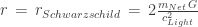 ) Black Hole Event Horizon, distance of the gradient gravity field
![{T_{Energy}}_{(\theta \phi)}\;=\; \frac{1}{4} ( \frac{c^4_{Light}}{G})[{r}(\frac{{\Omega_{Map}}_{(\theta \phi)}}{2\pi})]\,\,=\,\,\frac{1}{2}\,{m_{Net}\,c^2_{Light}}\,[\frac{({\Omega_{Map}}_{(\theta \phi)})^2}{2\,(ln(\frac{{c^2_{Light}}\,r}{2\,{m_{Net}}\,G}))^2\,\,+\,\,({\Omega_{Map}}_{(\theta \phi)})^2}]^2[(\frac{{\Omega_{Map}}_{(\theta \phi)}}{2\pi})]](https://s0.wp.com/latex.php?latex=%7BT_%7BEnergy%7D%7D_%7B%28%5Ctheta+%5Cphi%29%7D%5C%3B%3D%5C%3B+%5Cfrac%7B1%7D%7B4%7D+%28+%5Cfrac%7Bc%5E4_%7BLight%7D%7D%7BG%7D%29%5B%7Br%7D%28%5Cfrac%7B%7B%5COmega_%7BMap%7D%7D_%7B%28%5Ctheta+%5Cphi%29%7D%7D%7B2%5Cpi%7D%29%5D%5C%2C%5C%2C%3D%5C%2C%5C%2C%5Cfrac%7B1%7D%7B2%7D%5C%2C%7Bm_%7BNet%7D%5C%2Cc%5E2_%7BLight%7D%7D%5C%2C%5B%5Cfrac%7B%28%7B%5COmega_%7BMap%7D%7D_%7B%28%5Ctheta+%5Cphi%29%7D%29%5E2%7D%7B2%5C%2C%28ln%28%5Cfrac%7B%7Bc%5E2_%7BLight%7D%7D%5C%2Cr%7D%7B2%5C%2C%7Bm_%7BNet%7D%7D%5C%2CG%7D%29%29%5E2%5C%2C%5C%2C%2B%5C%2C%5C%2C%28%7B%5COmega_%7BMap%7D%7D_%7B%28%5Ctheta+%5Cphi%29%7D%29%5E2%7D%5D%5E2%5B%28%5Cfrac%7B%7B%5COmega_%7BMap%7D%7D_%7B%28%5Ctheta+%5Cphi%29%7D%7D%7B2%5Cpi%7D%29%5D&bg=ffffff&fg=333333&s=1&c=20201002)
![{{T_{Energy}}_{(\theta \phi)}}_{BH}\;=\,\,\frac{1}{2}\,{m_{Net}\,c^2_{Light}}\,[(\frac{{\Omega_{Map}}_{(\theta \phi)}}{2\pi})]](https://s0.wp.com/latex.php?latex=%7B%7BT_%7BEnergy%7D%7D_%7B%28%5Ctheta+%5Cphi%29%7D%7D_%7BBH%7D%5C%3B%3D%5C%2C%5C%2C%5Cfrac%7B1%7D%7B2%7D%5C%2C%7Bm_%7BNet%7D%5C%2Cc%5E2_%7BLight%7D%7D%5C%2C%5B%28%5Cfrac%7B%7B%5COmega_%7BMap%7D%7D_%7B%28%5Ctheta+%5Cphi%29%7D%7D%7B2%5Cpi%7D%29%5D&bg=ffffff&fg=333333&s=1&c=20201002)
************************************************************
![{{T_{Energy}}_{(\theta \phi)}}_{BH}\;\;=\;\;\frac{m_{Net}^2\,G}{r_{Schwarzschild}}\,[(\frac{{\Omega_{Map}}_{(\theta \phi)}}{2\pi})]](https://s0.wp.com/latex.php?latex=%7B%7BT_%7BEnergy%7D%7D_%7B%28%5Ctheta+%5Cphi%29%7D%7D_%7BBH%7D%5C%3B%5C%3B%3D%5C%3B%5C%3B%5Cfrac%7Bm_%7BNet%7D%5E2%5C%2CG%7D%7Br_%7BSchwarzschild%7D%7D%5C%2C%5B%28%5Cfrac%7B%7B%5COmega_%7BMap%7D%7D_%7B%28%5Ctheta+%5Cphi%29%7D%7D%7B2%5Cpi%7D%29%5D&bg=ffffff&fg=333333&s=1&c=20201002)
************************************************************
(3) The Total Mechanical Energy Conservation in direct relation to the – Einstein Field Equation of General Relativity
Total Mechanical Energy Conservation
Next, substituting the “Stress Kinetic Energy” into the above equation
![\frac{E_{Total}}{m_{Mass}}\,\,=\,\,\frac{1}{m_{Mass}}[{T_{Energy}}_{(\theta \phi)}(\frac{2\pi}{{\Omega_{Map}}_{(\theta \phi)}})\;\;+\;\;{V_{Gravity-Potential}}]](https://s0.wp.com/latex.php?latex=%5Cfrac%7BE_%7BTotal%7D%7D%7Bm_%7BMass%7D%7D%5C%2C%5C%2C%3D%5C%2C%5C%2C%5Cfrac%7B1%7D%7Bm_%7BMass%7D%7D%5B%7BT_%7BEnergy%7D%7D_%7B%28%5Ctheta+%5Cphi%29%7D%28%5Cfrac%7B2%5Cpi%7D%7B%7B%5COmega_%7BMap%7D%7D_%7B%28%5Ctheta+%5Cphi%29%7D%7D%29%5C%3B%5C%3B%2B%5C%3B%5C%3B%7BV_%7BGravity-Potential%7D%7D%5D&bg=ffffff&fg=333333&s=1&c=20201002)
************************************************************
Total Mechanical Energy Conservation – Einstein Field Equation
![\frac{{E_{Total}}_{(\theta \phi)}}{m_{Mass}}\,\,=\,\,\frac{1}{m_{Mass}}[ {T_{Energy}}_{(\theta \phi)}\;\;+\;\;{V_{Gravity-Potential}}[(\frac{{\Omega_{Map}}_{(\theta \phi)}}{2\pi})]]](https://s0.wp.com/latex.php?latex=%5Cfrac%7B%7BE_%7BTotal%7D%7D_%7B%28%5Ctheta+%5Cphi%29%7D%7D%7Bm_%7BMass%7D%7D%5C%2C%5C%2C%3D%5C%2C%5C%2C%5Cfrac%7B1%7D%7Bm_%7BMass%7D%7D%5B+%7BT_%7BEnergy%7D%7D_%7B%28%5Ctheta+%5Cphi%29%7D%5C%3B%5C%3B%2B%5C%3B%5C%3B%7BV_%7BGravity-Potential%7D%7D%5B%28%5Cfrac%7B%7B%5COmega_%7BMap%7D%7D_%7B%28%5Ctheta+%5Cphi%29%7D%7D%7B2%5Cpi%7D%29%5D%5D&bg=ffffff&fg=333333&s=1&c=20201002)
************************************************************
Total Mechanical Energy Conservation – Einstein Field Equation
![\frac{{E_{Total}}_{(\theta \phi)}}{m_{Mass}}=[\frac{1}{4}(\frac{c^4_{Light}}{m_{Mass}G})[\frac{1}{2\pi}[{R_{(\theta \phi)}}-{{g_{Vol}}_{(\theta \phi)}}(\frac{R_{Heat}}{2}-\Lambda_{Einstein})]]-\frac{m_{Net}\,G}{r}\,[(\frac{{\Omega_{Map}}_{(\theta \phi)}}{2\pi})]]](https://s0.wp.com/latex.php?latex=%5Cfrac%7B%7BE_%7BTotal%7D%7D_%7B%28%5Ctheta+%5Cphi%29%7D%7D%7Bm_%7BMass%7D%7D%3D%5B%5Cfrac%7B1%7D%7B4%7D%28%5Cfrac%7Bc%5E4_%7BLight%7D%7D%7Bm_%7BMass%7DG%7D%29%5B%5Cfrac%7B1%7D%7B2%5Cpi%7D%5B%7BR_%7B%28%5Ctheta+%5Cphi%29%7D%7D-%7B%7Bg_%7BVol%7D%7D_%7B%28%5Ctheta+%5Cphi%29%7D%7D%28%5Cfrac%7BR_%7BHeat%7D%7D%7B2%7D-%5CLambda_%7BEinstein%7D%29%5D%5D-%5Cfrac%7Bm_%7BNet%7D%5C%2CG%7D%7Br%7D%5C%2C%5B%28%5Cfrac%7B%7B%5COmega_%7BMap%7D%7D_%7B%28%5Ctheta+%5Cphi%29%7D%7D%7B2%5Cpi%7D%29%5D%5D&bg=ffffff&fg=333333&s=1&c=20201002)
************************************************************
Total Mechanical Energy Conservation – Einstein Field Equation
![\frac{{E_{Total}}_{(\theta \phi)}}{m_{Mass}}\,\,=\,\,[\frac{1}{2}\,(\frac{m_{Net}}{m_{Mass}})\,{c^2_{Light}}\,[\frac{({\Omega_{Map}}_{(\theta \phi)})^2}{2\,(ln(\frac{{c^2_{Light}}\,r}{2\,{m_{Net}}\,G}))^2\,\,+\,\,({\Omega_{Map}}_{(\theta \phi)})^2}]^2\,\,\,-\,\,\,\frac{m_{Net}\,G}{r}]\,[(\frac{{\Omega_{Map}}_{(\theta \phi)}}{2\pi})]](https://s0.wp.com/latex.php?latex=%5Cfrac%7B%7BE_%7BTotal%7D%7D_%7B%28%5Ctheta+%5Cphi%29%7D%7D%7Bm_%7BMass%7D%7D%5C%2C%5C%2C%3D%5C%2C%5C%2C%5B%5Cfrac%7B1%7D%7B2%7D%5C%2C%28%5Cfrac%7Bm_%7BNet%7D%7D%7Bm_%7BMass%7D%7D%29%5C%2C%7Bc%5E2_%7BLight%7D%7D%5C%2C%5B%5Cfrac%7B%28%7B%5COmega_%7BMap%7D%7D_%7B%28%5Ctheta+%5Cphi%29%7D%29%5E2%7D%7B2%5C%2C%28ln%28%5Cfrac%7B%7Bc%5E2_%7BLight%7D%7D%5C%2Cr%7D%7B2%5C%2C%7Bm_%7BNet%7D%7D%5C%2CG%7D%29%29%5E2%5C%2C%5C%2C%2B%5C%2C%5C%2C%28%7B%5COmega_%7BMap%7D%7D_%7B%28%5Ctheta+%5Cphi%29%7D%29%5E2%7D%5D%5E2%5C%2C%5C%2C%5C%2C-%5C%2C%5C%2C%5C%2C%5Cfrac%7Bm_%7BNet%7D%5C%2CG%7D%7Br%7D%5D%5C%2C%5B%28%5Cfrac%7B%7B%5COmega_%7BMap%7D%7D_%7B%28%5Ctheta+%5Cphi%29%7D%7D%7B2%5Cpi%7D%29%5D+&bg=ffffff&fg=333333&s=1&c=20201002)
************************************************************
(4) The Total Mechanical Energy Conservation – Energy States
The Total Mechanical Energy Conservation of a “Gradient Gravitational Field” of energy potentials, and the “Inertial Net Mass”, of the isolated system is described by a range of “Energy States”; given by the following conditional cases.

************************************************************
(Case #1) The Total Mechanical Energy Conservation – “Strongly Bound Condition” to a Gravitational Potential “Energy State”
In the case where “mass” and “energy” are in a “Bound/Strongly” condition to a “Gravitational Potential” of a gradient gravitational field, the Total Mechanical Energy Conservation ( ), is equal to the Gravitational Potential Energy located at a specific potential, of the gravity field gradient.
And the Net Kinetic Energy ( ), at that potential, is equal to zero (0).
************************************************************
Total Mechanical Energy Conservation
Next, substituting the, Net Kinetic Energy (), yields the Total Mechanical Energy Conservation given by;
Total Mechanical Energy Conservation – “Bound/Strongly” to Gravitational Field Condition


************************************************************
(Case #2) The Total Mechanical Energy Conservation – “Orbiting Condition” in Gravitational Potential “Energy State”
In the case where “mass” and “energy” are in “Orbiting” condition in a “Gravitational Potential” of a gradient gravitational field, the Total Mechanical Energy Conservation ( ) equals to one half the Gravitational (
 ) Potential Energy, and is equal to negative of the Kinetic Energy (
 ).
).
************************************************************
Total Mechanical Energy Conservation

Next, setting the Total Mechanical Energy Conservation “Orbital Energy” equals to one half the Gravitational Potential Energy (), and negative of the Kinetic Energy (), given by the following;

************************************************************

************************************************************
Gravitational Field – Mechanical “Orbital Energy” – where the Kinetic Energy () equals to negative one half the Gravitational Potential Energy (). Potential Energy Potentials.


************************************************************
Gravitational Field – Mechanical “Orbital Energy” – where the Kinetic Energy () equals to negative one half the Gravitational Potential Energy (). Kinetic Energy “Spacetime” Potentials.
![\frac{1}{2}{|\vec{v}|^2_{CM}}\;\;=\;\;\frac{1}{2}{v^2_{Gravity}}_{Spacetime}\;\;=\;\;\frac{1}{2}\,{c^2_{Light}}\,[\frac{({\Omega_{Map}}_{(\theta \phi)})^2}{2\,(ln(\frac{{c^2_{Light}}\,r}{2\,{m_{Net}}\,G}))^2\,\,+\,\,({\Omega_{Map}}_{(\theta \phi)})^2}]^2](https://s0.wp.com/latex.php?latex=%5Cfrac%7B1%7D%7B2%7D%7B%7C%5Cvec%7Bv%7D%7C%5E2_%7BCM%7D%7D%5C%3B%5C%3B%3D%5C%3B%5C%3B%5Cfrac%7B1%7D%7B2%7D%7Bv%5E2_%7BGravity%7D%7D_%7BSpacetime%7D%5C%3B%5C%3B%3D%5C%3B%5C%3B%5Cfrac%7B1%7D%7B2%7D%5C%2C%7Bc%5E2_%7BLight%7D%7D%5C%2C%5B%5Cfrac%7B%28%7B%5COmega_%7BMap%7D%7D_%7B%28%5Ctheta+%5Cphi%29%7D%29%5E2%7D%7B2%5C%2C%28ln%28%5Cfrac%7B%7Bc%5E2_%7BLight%7D%7D%5C%2Cr%7D%7B2%5C%2C%7Bm_%7BNet%7D%7D%5C%2CG%7D%29%29%5E2%5C%2C%5C%2C%2B%5C%2C%5C%2C%28%7B%5COmega_%7BMap%7D%7D_%7B%28%5Ctheta+%5Cphi%29%7D%29%5E2%7D%5D%5E2&bg=ffffff&fg=333333&s=1&c=20201002)
************************************************************
(Case #3) The Total Mechanical Energy Conservation – “Minimum Escape Condition” to “Unbound” from a Gravitational Potential “Energy State”
In the case where “mass” and “energy” are in “Minimum Escape” condition to “Unbound” from a “Gravitational Potential” of a gradient gravitational field, the Total Mechanical Energy Conservation is equal to zero ( ) .
) .
In the case where “mass” and “energy” are in “Minimum Escape” condition, this is also known as the “Escape Energy” condition, and is a measure of the “Escape Velocity” from a “Gradient Gravitational Field Potential”; and the Net Kinetic Energy equals to negative of the Gravitational Potential Energy ( ), and located at a specific potential, of the gravity field gradient.
************************************************************
Total Mechanical Energy Conservation
Next, setting the Total Mechanical Energy Conservation “Escape Energy” equal to zero (0) is given by the following;
************************************************************
Gravitational Field – Mechanical “Minimum Escape Energy” – equals to Gradient Gravitational Field “Potential Energy” Potentials


************************************************************
The Escape Velocity from a local gravitational “Potential Energy” potential is then given by:


************************************************************
Gravitational Field – Mechanical “Minimum Escape Energy” – equals to Gradient Gravitational Field “Kinetic Energy” Vacuum of Space-time Potentials
![\frac{1}{2}{|\vec{v}|^2_{CM}}\;\;=\;\;{v^2_{Gravity}}_{Spacetime}\;\;=\;\;\frac{1}{2}\,{c^2_{Light}}\,[\frac{({\Omega_{Map}}_{(\theta \phi)})^2}{2\,(ln(\frac{{c^2_{Light}}\,r}{2\,{m_{Net}}\,G}))^2\,\,+\,\,({\Omega_{Map}}_{(\theta \phi)})^2}]^2](https://s0.wp.com/latex.php?latex=%5Cfrac%7B1%7D%7B2%7D%7B%7C%5Cvec%7Bv%7D%7C%5E2_%7BCM%7D%7D%5C%3B%5C%3B%3D%5C%3B%5C%3B%7Bv%5E2_%7BGravity%7D%7D_%7BSpacetime%7D%5C%3B%5C%3B%3D%5C%3B%5C%3B%5Cfrac%7B1%7D%7B2%7D%5C%2C%7Bc%5E2_%7BLight%7D%7D%5C%2C%5B%5Cfrac%7B%28%7B%5COmega_%7BMap%7D%7D_%7B%28%5Ctheta+%5Cphi%29%7D%29%5E2%7D%7B2%5C%2C%28ln%28%5Cfrac%7B%7Bc%5E2_%7BLight%7D%7D%5C%2Cr%7D%7B2%5C%2C%7Bm_%7BNet%7D%7D%5C%2CG%7D%29%29%5E2%5C%2C%5C%2C%2B%5C%2C%5C%2C%28%7B%5COmega_%7BMap%7D%7D_%7B%28%5Ctheta+%5Cphi%29%7D%29%5E2%7D%5D%5E2&bg=ffffff&fg=333333&s=1&c=20201002)
************************************************************
The Escape Velocity from a local gravitational “Kinetic Energy” space-time potential is then given by:
![{|\vec{v}|_{CM}}\,\,=\,\,{v_{Gravity}}_{Spacetime}\,\sqrt{2}\,\,=\,\,(-){c_{Light}}\,[\frac{({\Omega_{Map}}_{(\theta \phi)})^2}{2\,(ln(\frac{{c^2_{Light}}\,r}{2\,{m_{Net}}\,G}))^2\,\,+\,\,({\Omega_{Map}}_{(\theta \phi)})^2}]](https://s0.wp.com/latex.php?latex=%7B%7C%5Cvec%7Bv%7D%7C_%7BCM%7D%7D%5C%2C%5C%2C%3D%5C%2C%5C%2C%7Bv_%7BGravity%7D%7D_%7BSpacetime%7D%5C%2C%5Csqrt%7B2%7D%5C%2C%5C%2C%3D%5C%2C%5C%2C%28-%29%7Bc_%7BLight%7D%7D%5C%2C%5B%5Cfrac%7B%28%7B%5COmega_%7BMap%7D%7D_%7B%28%5Ctheta+%5Cphi%29%7D%29%5E2%7D%7B2%5C%2C%28ln%28%5Cfrac%7B%7Bc%5E2_%7BLight%7D%7D%5C%2Cr%7D%7B2%5C%2C%7Bm_%7BNet%7D%7D%5C%2CG%7D%29%29%5E2%5C%2C%5C%2C%2B%5C%2C%5C%2C%28%7B%5COmega_%7BMap%7D%7D_%7B%28%5Ctheta+%5Cphi%29%7D%29%5E2%7D%5D&bg=ffffff&fg=333333&s=1&c=20201002)
************************************************************
(Case #4) The Total Mechanical Energy Conservation – “Totally Free Condition” from Gravitational “Potential Energy” – “Kinetic Energy” State Potentials
In the case where “mass” and “energy” are in “Totally Free Condition” from a “Gravitational Potential”, and from the “gravitational attraction” effects, of a gradient gravitational field. This energy state is complete kinetic energy, where the Total Mechanical Energy Conservation ( ), is equal to the Net Kinetic Energy located at specific “Kinetic Energy Potentials”, of the gravity field gradient, relative to the “Schwarzschild Radius” () “Black Hole Event Horizon”; which is located at the core, the most minimum distance and volume of the gradient field.
And the Gravitational Potential Energy ( ), at that potential, is equal to zero (0).
************************************************************
Total Mechanical Energy Conservation

Next, substituting the, Gravitational Potential Energy (), yields the Total Mechanical Energy Conservation at specific “Kinetic Energy Potentials”, given by the following;
Total Mechanical Energy Conservation – “Totally Free” from Gravitational Potential Energy Condition – Kinetic Energy Potentials

![\frac{E_{Self-Total}}{m_{Net}}\,\,=\,\,\frac{E_{Total}}{m_{mass}}\,\,=\,\,\frac{1}{2}{|\vec{v}|^2_{CM}}\,\,=\,\,\frac{1}{2}\,{c^2_{Light}}\,[\frac{({\Omega_{Map}}_{(\theta \phi)})^2}{2\,(ln(\frac{{c^2_{Light}}\,r}{2\,{m_{Net}}\,G}))^2\,\,+\,\,({\Omega_{Map}}_{(\theta \phi)})^2}]^2](https://s0.wp.com/latex.php?latex=%5Cfrac%7BE_%7BSelf-Total%7D%7D%7Bm_%7BNet%7D%7D%5C%2C%5C%2C%3D%5C%2C%5C%2C%5Cfrac%7BE_%7BTotal%7D%7D%7Bm_%7Bmass%7D%7D%5C%2C%5C%2C%3D%5C%2C%5C%2C%5Cfrac%7B1%7D%7B2%7D%7B%7C%5Cvec%7Bv%7D%7C%5E2_%7BCM%7D%7D%5C%2C%5C%2C%3D%5C%2C%5C%2C%5Cfrac%7B1%7D%7B2%7D%5C%2C%7Bc%5E2_%7BLight%7D%7D%5C%2C%5B%5Cfrac%7B%28%7B%5COmega_%7BMap%7D%7D_%7B%28%5Ctheta+%5Cphi%29%7D%29%5E2%7D%7B2%5C%2C%28ln%28%5Cfrac%7B%7Bc%5E2_%7BLight%7D%7D%5C%2Cr%7D%7B2%5C%2C%7Bm_%7BNet%7D%7D%5C%2CG%7D%29%29%5E2%5C%2C%5C%2C%2B%5C%2C%5C%2C%28%7B%5COmega_%7BMap%7D%7D_%7B%28%5Ctheta+%5Cphi%29%7D%29%5E2%7D%5D%5E2&bg=ffffff&fg=333333&s=1&c=20201002)
************************************************************
The Escape Velocity from a local gravitational “Kinetic Energy” potential is then given by:
![{|\vec{v}|_{CM}}\,\,=\,\,(-){c_{Light}}\,[\frac{({\Omega_{Map}}_{(\theta \phi)})^2}{2\,(ln(\frac{{c^2_{Light}}\,r}{2\,{m_{Net}}\,G}))^2\,\,+\,\,({\Omega_{Map}}_{(\theta \phi)})^2}]](https://s0.wp.com/latex.php?latex=%7B%7C%5Cvec%7Bv%7D%7C_%7BCM%7D%7D%5C%2C%5C%2C%3D%5C%2C%5C%2C%28-%29%7Bc_%7BLight%7D%7D%5C%2C%5B%5Cfrac%7B%28%7B%5COmega_%7BMap%7D%7D_%7B%28%5Ctheta+%5Cphi%29%7D%29%5E2%7D%7B2%5C%2C%28ln%28%5Cfrac%7B%7Bc%5E2_%7BLight%7D%7D%5C%2Cr%7D%7B2%5C%2C%7Bm_%7BNet%7D%7D%5C%2CG%7D%29%29%5E2%5C%2C%5C%2C%2B%5C%2C%5C%2C%28%7B%5COmega_%7BMap%7D%7D_%7B%28%5Ctheta+%5Cphi%29%7D%29%5E2%7D%5D&bg=ffffff&fg=333333&s=1&c=20201002)
************************************************************
The above “New” equation for describing the condition when the “The Total Mechanical Energy” is equal to the “Total Kinetic Energy” for any “mass” or “energy”, located at any potential of the gradient gravitational field; although the “mass” or “energy”, is totally free from the gravitating influences of the field. The energy potentials in this conditions are “Kinetic Energy Potentials”.
The above equation allows for prediction of the “Total Kinetic Energy” at each potential of the gradient gravitational field, located at some distace relative to the, “Black Hole Event Horizon” “Schwarzschild Radius” ().
This “energy state” condition, is free from “gravitational attraction” influences! This is therefore a gradient field of “Kinetic Energy” Potentials, and not a gradient field of “Potential Energy” Potentials.
************************************************************
(Case #5) The Total Mechanical Energy Conservation – “Partially/Weakly Bound Condition” to a Gravitational Potential “Energy State”
In the case where “mass” and “energy” are in “Partially/Weakly Bound” condition to a “Gravitational Potential” of “Potential Energy” of a gradient gravitational field, the Total Mechanical Energy Conservation () is equal to the net sum of the Net Kinetic Energy plus the Gravitational Potential Energy, located at each potential of the gradient gravity field.
The “Partially/Weakly Bound” condition in a gravitational potential, is where there is sufficient energy to escape the field, yet remains very loosely bound to the, “Gradient Gravitational Field Potential”.
In the “Partially/Weakly Bound” condition in a gravitational potential, the Net Kinetic Energy is greater than or equal to negative of the Gravitational Potential Energy ( ) located at a specific potential, of the gravity field gradient.
************************************************************
Total Mechanical Energy Conservation
************************************************************
Total Mechanical Energy Conservation – “Partially/Weakly Bound” to Gravitational Potential Energy Condition

************************************************************
![\frac{E_{Self-Total}}{m_{Net}}\,\,=\,\,\frac{E_{Total}}{m_{mass}}\;\;=\;\;[\frac{1}{2}{|\vec{v}|^2_{CM}}\;\;-\;\;\frac{m_{Net}\,G}{r}]](https://s0.wp.com/latex.php?latex=%5Cfrac%7BE_%7BSelf-Total%7D%7D%7Bm_%7BNet%7D%7D%5C%2C%5C%2C%3D%5C%2C%5C%2C%5Cfrac%7BE_%7BTotal%7D%7D%7Bm_%7Bmass%7D%7D%5C%3B%5C%3B%3D%5C%3B%5C%3B%5B%5Cfrac%7B1%7D%7B2%7D%7B%7C%5Cvec%7Bv%7D%7C%5E2_%7BCM%7D%7D%5C%3B%5C%3B-%5C%3B%5C%3B%5Cfrac%7Bm_%7BNet%7D%5C%2CG%7D%7Br%7D%5D&bg=ffffff&fg=333333&s=1&c=20201002)
![\frac{E_{Self-Total}}{m_{Net}}\,\,=\,\,\frac{E_{Total}}{m_{mass}}\,\,=\,\,[\frac{1}{2}\,{c^2_{Light}}\,[\frac{({\Omega_{Map}}_{(\theta \phi)})^2}{2\,(ln(\frac{{c^2_{Light}}\,r}{2\,{m_{Net}}\,G}))^2\,\,+\,\,({\Omega_{Map}}_{(\theta \phi)})^2}]^2\,\,\,-\,\,\,\frac{m_{Net}\,G}{r}]](https://s0.wp.com/latex.php?latex=%5Cfrac%7BE_%7BSelf-Total%7D%7D%7Bm_%7BNet%7D%7D%5C%2C%5C%2C%3D%5C%2C%5C%2C%5Cfrac%7BE_%7BTotal%7D%7D%7Bm_%7Bmass%7D%7D%5C%2C%5C%2C%3D%5C%2C%5C%2C%5B%5Cfrac%7B1%7D%7B2%7D%5C%2C%7Bc%5E2_%7BLight%7D%7D%5C%2C%5B%5Cfrac%7B%28%7B%5COmega_%7BMap%7D%7D_%7B%28%5Ctheta+%5Cphi%29%7D%29%5E2%7D%7B2%5C%2C%28ln%28%5Cfrac%7B%7Bc%5E2_%7BLight%7D%7D%5C%2Cr%7D%7B2%5C%2C%7Bm_%7BNet%7D%7D%5C%2CG%7D%29%29%5E2%5C%2C%5C%2C%2B%5C%2C%5C%2C%28%7B%5COmega_%7BMap%7D%7D_%7B%28%5Ctheta+%5Cphi%29%7D%29%5E2%7D%5D%5E2%5C%2C%5C%2C%5C%2C-%5C%2C%5C%2C%5C%2C%5Cfrac%7Bm_%7BNet%7D%5C%2CG%7D%7Br%7D%5D&bg=ffffff&fg=333333&s=1&c=20201002)
************************************************************
General Constants
Gravitational Universal Constant

Speed of Light in vacuum constant

Cosmic “Dark” Vacuum Force universal constant

Black Hole Linear Mass Density

************************************************************
Closing Remarks:
The above work discusses a new set of equations for describing the, “Total Mechanical Energy Conservation” of an isolated system body in regards to specific “Energy States” of various “Potential Energy Potentials” and “Kinetic Energy Potentials”. The above energy equations were also described in terms of the “Einstein Field Equation”, the “Universal Cosmic “Dark” Vacuum Force”, and the “Vacuum Energy”.
The “Einstein Field Equation” and the “Vacuum Energy” was shown to be an “Elastic “Stress” Kinetic Energy” equation that predicts that there are “Kinetic Energy Potentials”, and a warping, deforming, and curving of space and time in the vacuum, and in the local vicinity of any mass object.
The “Net Inertial Mass” was shown conceptualy and mathematically, to warp space and time, and create a gradient energy field of “Potential” and “Kinetic” energy potentials surrounding the mass object. And, at the core of the gradient field of potentials is the “Black Hole Event Horizon”, having a specific “Schwarzschild” “Radius” and “Volume”.
It is at the core of the gradient gravity field, the location of the “Black Hole Event Horizon”, which is the lowest potential of the gradient field, and the source of gravitation, where “mass” and “space” of an orgainzed unit or system body, are in universal continuum.
************************************************************
Citation
Cite this article as:
Robert Louis Kemp; The Super Principia Mathematica – The Rage to Master Conceptual & Mathematical Physics – The General Theory of Relativity – “Total Mechanical Energy Conservation – Escape Velocity & Binding Energy – Einstein Field Equation” – Online Volume – ISBN 978-0-9841518-2-0, Volume 3; July 2010
************************************************************
Best,
All Comments are welcome.
Author: Robert Louis Kemp
http://www.SuperPrincipia.com


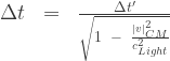
![\Delta{t'}\;\;=\;\;\frac{\Delta{t}\;\;-\;\; \Delta{\tau_{Sync}}}{\sqrt{1 \;\;-\;\; \frac{{|v|^2_{CM}}}{{c^2_{Light}}}}}\;\;=\;\;\frac{\Delta{t}\;\;-\;\; [\frac{\vec{|v|_{CM}}\;\;\vec{u_{Frame}}}{c^2_{Light}}]\;\Delta{t}}{\sqrt{1 \;\;-\;\; \frac{{|v|^2_{CM}}}{{c^2_{Light}}}}}](https://s0.wp.com/latex.php?latex=%5CDelta%7Bt%27%7D%5C%3B%5C%3B%3D%5C%3B%5C%3B%5Cfrac%7B%5CDelta%7Bt%7D%5C%3B%5C%3B-%5C%3B%5C%3B+%5CDelta%7B%5Ctau_%7BSync%7D%7D%7D%7B%5Csqrt%7B1+%5C%3B%5C%3B-%5C%3B%5C%3B+%5Cfrac%7B%7B%7Cv%7C%5E2_%7BCM%7D%7D%7D%7B%7Bc%5E2_%7BLight%7D%7D%7D%7D%7D%5C%3B%5C%3B%3D%5C%3B%5C%3B%5Cfrac%7B%5CDelta%7Bt%7D%5C%3B%5C%3B-%5C%3B%5C%3B+%5B%5Cfrac%7B%5Cvec%7B%7Cv%7C_%7BCM%7D%7D%5C%3B%5C%3B%5Cvec%7Bu_%7BFrame%7D%7D%7D%7Bc%5E2_%7BLight%7D%7D%5D%5C%3B%5CDelta%7Bt%7D%7D%7B%5Csqrt%7B1+%5C%3B%5C%3B-%5C%3B%5C%3B+%5Cfrac%7B%7B%7Cv%7C%5E2_%7BCM%7D%7D%7D%7B%7Bc%5E2_%7BLight%7D%7D%7D%7D%7D&bg=ffffff&fg=333333&s=1&c=20201002)
![\Delta{t'}\;\;=\;\;\frac{\Delta{t}\;\;-\;\; [\frac{\vec{|v|_{CM}}}{c^2_{Light}}]\;\;\vec{r}}{\sqrt{1 \;\;-\;\; \frac{{|v|^2_{CM}}}{{c^2_{Light}}}}}](https://s0.wp.com/latex.php?latex=%5CDelta%7Bt%27%7D%5C%3B%5C%3B%3D%5C%3B%5C%3B%5Cfrac%7B%5CDelta%7Bt%7D%5C%3B%5C%3B-%5C%3B%5C%3B+%5B%5Cfrac%7B%5Cvec%7B%7Cv%7C_%7BCM%7D%7D%7D%7Bc%5E2_%7BLight%7D%7D%5D%5C%3B%5C%3B%5Cvec%7Br%7D%7D%7B%5Csqrt%7B1+%5C%3B%5C%3B-%5C%3B%5C%3B+%5Cfrac%7B%7B%7Cv%7C%5E2_%7BCM%7D%7D%7D%7B%7Bc%5E2_%7BLight%7D%7D%7D%7D%7D&bg=ffffff&fg=333333&s=1&c=20201002)

![\vec{x'}\;\;=\;\;\frac{\vec{x}\;\;-\;\; {\vec{|v|_{CM(x)}}\;\Delta{t}}}{\sqrt{1 \;\;-\;\; \frac{[ {|v|^2_{CM(x)}} \;\;+\;\; {|v|^2_{CM(y)}} \;\;+\;\;{|v|^2_{CM(z)}}]}{{c^2_{Light}}}}}](https://s0.wp.com/latex.php?latex=%5Cvec%7Bx%27%7D%5C%3B%5C%3B%3D%5C%3B%5C%3B%5Cfrac%7B%5Cvec%7Bx%7D%5C%3B%5C%3B-%5C%3B%5C%3B+%7B%5Cvec%7B%7Cv%7C_%7BCM%28x%29%7D%7D%5C%3B%5CDelta%7Bt%7D%7D%7D%7B%5Csqrt%7B1+%5C%3B%5C%3B-%5C%3B%5C%3B+%5Cfrac%7B%5B+%7B%7Cv%7C%5E2_%7BCM%28x%29%7D%7D+%5C%3B%5C%3B%2B%5C%3B%5C%3B+%7B%7Cv%7C%5E2_%7BCM%28y%29%7D%7D+%5C%3B%5C%3B%2B%5C%3B%5C%3B%7B%7Cv%7C%5E2_%7BCM%28z%29%7D%7D%5D%7D%7B%7Bc%5E2_%7BLight%7D%7D%7D%7D%7D&bg=ffffff&fg=333333&s=1&c=20201002)
![\vec{y'}\;\;=\;\;\frac{\vec{y}\;\;-\;\; {\vec{|v|_{CM(y)}}\;\Delta{t}}}{\sqrt{1 \;\;-\;\; \frac{[ {|v|^2_{CM(x)}} \;\;+\;\; {|v|^2_{CM(y)}} \;\;+\;\;{|v|^2_{CM(z)}}]}{{c^2_{Light}}}}}](https://s0.wp.com/latex.php?latex=%5Cvec%7By%27%7D%5C%3B%5C%3B%3D%5C%3B%5C%3B%5Cfrac%7B%5Cvec%7By%7D%5C%3B%5C%3B-%5C%3B%5C%3B+%7B%5Cvec%7B%7Cv%7C_%7BCM%28y%29%7D%7D%5C%3B%5CDelta%7Bt%7D%7D%7D%7B%5Csqrt%7B1+%5C%3B%5C%3B-%5C%3B%5C%3B+%5Cfrac%7B%5B+%7B%7Cv%7C%5E2_%7BCM%28x%29%7D%7D+%5C%3B%5C%3B%2B%5C%3B%5C%3B+%7B%7Cv%7C%5E2_%7BCM%28y%29%7D%7D+%5C%3B%5C%3B%2B%5C%3B%5C%3B%7B%7Cv%7C%5E2_%7BCM%28z%29%7D%7D%5D%7D%7B%7Bc%5E2_%7BLight%7D%7D%7D%7D%7D&bg=ffffff&fg=333333&s=1&c=20201002)
![\vec{z'}\;\;=\;\;\frac{\vec{z}\;\;-\;\; {\vec{|v|_{CM(z)}}\;\Delta{t}}}{\sqrt{1 \;\;-\;\; \frac{[ {|v|^2_{CM(x)}} \;\;+\;\; {|v|^2_{CM(y)}} \;\;+\;\;{|v|^2_{CM(z)}}]}{{c^2_{Light}}}}}](https://s0.wp.com/latex.php?latex=%5Cvec%7Bz%27%7D%5C%3B%5C%3B%3D%5C%3B%5C%3B%5Cfrac%7B%5Cvec%7Bz%7D%5C%3B%5C%3B-%5C%3B%5C%3B+%7B%5Cvec%7B%7Cv%7C_%7BCM%28z%29%7D%7D%5C%3B%5CDelta%7Bt%7D%7D%7D%7B%5Csqrt%7B1+%5C%3B%5C%3B-%5C%3B%5C%3B+%5Cfrac%7B%5B+%7B%7Cv%7C%5E2_%7BCM%28x%29%7D%7D+%5C%3B%5C%3B%2B%5C%3B%5C%3B+%7B%7Cv%7C%5E2_%7BCM%28y%29%7D%7D+%5C%3B%5C%3B%2B%5C%3B%5C%3B%7B%7Cv%7C%5E2_%7BCM%28z%29%7D%7D%5D%7D%7B%7Bc%5E2_%7BLight%7D%7D%7D%7D%7D&bg=ffffff&fg=333333&s=1&c=20201002)
![\Delta{t}\;\;=\;\;\frac{\Delta{t'}\;\;+\;\; \Delta{\tau'_{Sync}}}{\sqrt{1 \;\;-\;\; \frac{{|v|^2_{CM}}}{{c^2_{Light}}}}}\;\;=\;\;\frac{\Delta{t'}\;\;+\;\; [\frac{\vec{|v|_{CM}}\;\;\vec{u'_{Frame}}}{c^2_{Light}}]\;\Delta{t'}}{\sqrt{1 \;\;-\;\; \frac{{|v|^2_{CM}}}{{c^2_{Light}}}}}](https://s0.wp.com/latex.php?latex=%5CDelta%7Bt%7D%5C%3B%5C%3B%3D%5C%3B%5C%3B%5Cfrac%7B%5CDelta%7Bt%27%7D%5C%3B%5C%3B%2B%5C%3B%5C%3B+%5CDelta%7B%5Ctau%27_%7BSync%7D%7D%7D%7B%5Csqrt%7B1+%5C%3B%5C%3B-%5C%3B%5C%3B+%5Cfrac%7B%7B%7Cv%7C%5E2_%7BCM%7D%7D%7D%7B%7Bc%5E2_%7BLight%7D%7D%7D%7D%7D%5C%3B%5C%3B%3D%5C%3B%5C%3B%5Cfrac%7B%5CDelta%7Bt%27%7D%5C%3B%5C%3B%2B%5C%3B%5C%3B+%5B%5Cfrac%7B%5Cvec%7B%7Cv%7C_%7BCM%7D%7D%5C%3B%5C%3B%5Cvec%7Bu%27_%7BFrame%7D%7D%7D%7Bc%5E2_%7BLight%7D%7D%5D%5C%3B%5CDelta%7Bt%27%7D%7D%7B%5Csqrt%7B1+%5C%3B%5C%3B-%5C%3B%5C%3B+%5Cfrac%7B%7B%7Cv%7C%5E2_%7BCM%7D%7D%7D%7B%7Bc%5E2_%7BLight%7D%7D%7D%7D%7D&bg=ffffff&fg=333333&s=1&c=20201002)
![\Delta{t}\;\;=\;\;\frac{\Delta{t'}\;\;+\;\; [\frac{\vec{|v|_{CM}}}{c^2_{Light}}]\;\;\vec{r'}}{\sqrt{1 \;\;-\;\; \frac{{|v|^2_{CM}}}{{c^2_{Light}}}}}](https://s0.wp.com/latex.php?latex=%5CDelta%7Bt%7D%5C%3B%5C%3B%3D%5C%3B%5C%3B%5Cfrac%7B%5CDelta%7Bt%27%7D%5C%3B%5C%3B%2B%5C%3B%5C%3B+%5B%5Cfrac%7B%5Cvec%7B%7Cv%7C_%7BCM%7D%7D%7D%7Bc%5E2_%7BLight%7D%7D%5D%5C%3B%5C%3B%5Cvec%7Br%27%7D%7D%7B%5Csqrt%7B1+%5C%3B%5C%3B-%5C%3B%5C%3B+%5Cfrac%7B%7B%7Cv%7C%5E2_%7BCM%7D%7D%7D%7B%7Bc%5E2_%7BLight%7D%7D%7D%7D%7D&bg=ffffff&fg=333333&s=1&c=20201002)

![\vec{x}\;\;=\;\;\frac{\vec{x'}\;\;+\;\; {\vec{|v|_{CM(x)}}\;\Delta{t'}}}{\sqrt{1 \;\;-\;\; \frac{[ {|v|^2_{CM(x)}} \;\;+\;\; {|v|^2_{CM(y)}}\;\;+ \;\;{|v|^2_{CM(z)}}]}{{c^2_{Light}}}}}](https://s0.wp.com/latex.php?latex=%5Cvec%7Bx%7D%5C%3B%5C%3B%3D%5C%3B%5C%3B%5Cfrac%7B%5Cvec%7Bx%27%7D%5C%3B%5C%3B%2B%5C%3B%5C%3B+%7B%5Cvec%7B%7Cv%7C_%7BCM%28x%29%7D%7D%5C%3B%5CDelta%7Bt%27%7D%7D%7D%7B%5Csqrt%7B1+%5C%3B%5C%3B-%5C%3B%5C%3B+%5Cfrac%7B%5B+%7B%7Cv%7C%5E2_%7BCM%28x%29%7D%7D+%5C%3B%5C%3B%2B%5C%3B%5C%3B+%7B%7Cv%7C%5E2_%7BCM%28y%29%7D%7D%5C%3B%5C%3B%2B+%5C%3B%5C%3B%7B%7Cv%7C%5E2_%7BCM%28z%29%7D%7D%5D%7D%7B%7Bc%5E2_%7BLight%7D%7D%7D%7D%7D&bg=ffffff&fg=333333&s=1&c=20201002)
![\vec{y}\;\;=\;\;\frac{\vec{y'}\;\;+\;\; {\vec{|v|_{CM(y)}}\;\Delta{t'}}}{\sqrt{1 \;\;-\;\; \frac{[ {|v|^2_{CM(x)}} \;\;+\;\; {|v|^2_{CM(y)}}\;\;+ \;\;{|v|^2_{CM(z)}}]}{{c^2_{Light}}}}}](https://s0.wp.com/latex.php?latex=%5Cvec%7By%7D%5C%3B%5C%3B%3D%5C%3B%5C%3B%5Cfrac%7B%5Cvec%7By%27%7D%5C%3B%5C%3B%2B%5C%3B%5C%3B+%7B%5Cvec%7B%7Cv%7C_%7BCM%28y%29%7D%7D%5C%3B%5CDelta%7Bt%27%7D%7D%7D%7B%5Csqrt%7B1+%5C%3B%5C%3B-%5C%3B%5C%3B+%5Cfrac%7B%5B+%7B%7Cv%7C%5E2_%7BCM%28x%29%7D%7D+%5C%3B%5C%3B%2B%5C%3B%5C%3B+%7B%7Cv%7C%5E2_%7BCM%28y%29%7D%7D%5C%3B%5C%3B%2B+%5C%3B%5C%3B%7B%7Cv%7C%5E2_%7BCM%28z%29%7D%7D%5D%7D%7B%7Bc%5E2_%7BLight%7D%7D%7D%7D%7D&bg=ffffff&fg=333333&s=1&c=20201002)
![\vec{z}\;\;=\;\;\frac{\vec{z'}\;\;+\;\; {\vec{|v|_{CM(z)}}\;\Delta{t'}}}{\sqrt{1 \;\;-\;\; \frac{[ {|v|^2_{CM(x)}} \;\;+\;\; {|v|^2_{CM(y)}} \;\;+\;\;{|v|^2_{CM(z)}}]}{{c^2_{Light}}}}}](https://s0.wp.com/latex.php?latex=%5Cvec%7Bz%7D%5C%3B%5C%3B%3D%5C%3B%5C%3B%5Cfrac%7B%5Cvec%7Bz%27%7D%5C%3B%5C%3B%2B%5C%3B%5C%3B+%7B%5Cvec%7B%7Cv%7C_%7BCM%28z%29%7D%7D%5C%3B%5CDelta%7Bt%27%7D%7D%7D%7B%5Csqrt%7B1+%5C%3B%5C%3B-%5C%3B%5C%3B+%5Cfrac%7B%5B+%7B%7Cv%7C%5E2_%7BCM%28x%29%7D%7D+%5C%3B%5C%3B%2B%5C%3B%5C%3B+%7B%7Cv%7C%5E2_%7BCM%28y%29%7D%7D+%5C%3B%5C%3B%2B%5C%3B%5C%3B%7B%7Cv%7C%5E2_%7BCM%28z%29%7D%7D%5D%7D%7B%7Bc%5E2_%7BLight%7D%7D%7D%7D%7D&bg=ffffff&fg=333333&s=1&c=20201002)

 ) be the power input or output the system; and is defined as the rate at which energy is input or output the system. Thus, the value of the “Power Outflow” (
 ) is negative if energy is flowing out of the system; and the “Power Inflow” (
 ) is positive if energy is flowing into of the system.
 ), multiplied by one half the square of the
  ) of an isolated system body; given by the following equation.

![{m_{Net}}\, \,=\,\,\displaystyle\sum_{i=1}^N {m_{i}}\,\,=\,\,[ {m_{1}} + {m_{2}} + {m_{3}} + ...... + {m_{N}}]\,\,](https://s0.wp.com/latex.php?latex=%7Bm_%7BNet%7D%7D%5C%2C+%5C%2C%3D%5C%2C%5C%2C%5Cdisplaystyle%5Csum_%7Bi%3D1%7D%5EN+%7Bm_%7Bi%7D%7D%5C%2C%5C%2C%3D%5C%2C%5C%2C%5B+%7Bm_%7B1%7D%7D+%2B+%7Bm_%7B2%7D%7D+%2B+%7Bm_%7B3%7D%7D+%2B+......+%2B+%7Bm_%7BN%7D%7D%5D%5C%2C%5C%2C&bg=ffffff&fg=333333&s=1&c=20201002)

 ) – in the
 ) – in the


 ) – of the mass bodies of a net mass system is a vector quantity, that describes direction dependent motion, or “Anisotropic Motion”, and measures “equal distance changing in equal times” motion of an isolated system mass body; and is described in two ways:
 ) divided by the


![{E_{Total}}\,\,=\,\,[\frac{1}{2}{m_{mass}}{|\vec{v}|^2_{CM}}\;\;-\;\;\frac{{m_{mass}\,m_{Net}\,G}}{r}]](https://s0.wp.com/latex.php?latex=%7BE_%7BTotal%7D%7D%5C%2C%5C%2C%3D%5C%2C%5C%2C%5B%5Cfrac%7B1%7D%7B2%7D%7Bm_%7Bmass%7D%7D%7B%7C%5Cvec%7Bv%7D%7C%5E2_%7BCM%7D%7D%5C%3B%5C%3B-%5C%3B%5C%3B%5Cfrac%7B%7Bm_%7Bmass%7D%5C%2Cm_%7BNet%7D%5C%2CG%7D%7D%7Br%7D%5D&bg=ffffff&fg=333333&s=1&c=20201002)
![{E_{Total}}\,\,=\,\,{m_{mass}}[\frac{1}{2}{|\vec{v}|^2_{CM}}\,\,-\,\,{g_{Gravity}}\,{r}]](https://s0.wp.com/latex.php?latex=%7BE_%7BTotal%7D%7D%5C%2C%5C%2C%3D%5C%2C%5C%2C%7Bm_%7Bmass%7D%7D%5B%5Cfrac%7B1%7D%7B2%7D%7B%7C%5Cvec%7Bv%7D%7C%5E2_%7BCM%7D%7D%5C%2C%5C%2C-%5C%2C%5C%2C%7Bg_%7BGravity%7D%7D%5C%2C%7Br%7D%5D&bg=ffffff&fg=333333&s=1&c=20201002)
![{E_{Total}}\,\,=\,\,\,{m_{mass}} [\frac{1}{2}{|\vec{v}|^2_{CM}}\,\,-\,\,{v^2_{Gravity}}]](https://s0.wp.com/latex.php?latex=%7BE_%7BTotal%7D%7D%5C%2C%5C%2C%3D%5C%2C%5C%2C%5C%2C%7Bm_%7Bmass%7D%7D+%5B%5Cfrac%7B1%7D%7B2%7D%7B%7C%5Cvec%7Bv%7D%7C%5E2_%7BCM%7D%7D%5C%2C%5C%2C-%5C%2C%5C%2C%7Bv%5E2_%7BGravity%7D%7D%5D&bg=ffffff&fg=333333&s=1&c=20201002)
![{E_{Total}}\,\,=\,\,[\frac{1}{2}{{m_{mass}}\,c^2_{Light}}\,[\frac{({\Omega_{Map}}_{(\theta \phi)})^2}{2\,(ln(\frac{{c^2_{Light}}\,r}{2\,{m_{Net}}\,G}))^2\;\;+\;\;({\Omega_{Map}}_{(\theta \phi)})^2}]^2\;\;-\;\;\frac{{m_{mass}\,m_{Net}\,G}}{r}]](https://s0.wp.com/latex.php?latex=%7BE_%7BTotal%7D%7D%5C%2C%5C%2C%3D%5C%2C%5C%2C%5B%5Cfrac%7B1%7D%7B2%7D%7B%7Bm_%7Bmass%7D%7D%5C%2Cc%5E2_%7BLight%7D%7D%5C%2C%5B%5Cfrac%7B%28%7B%5COmega_%7BMap%7D%7D_%7B%28%5Ctheta+%5Cphi%29%7D%29%5E2%7D%7B2%5C%2C%28ln%28%5Cfrac%7B%7Bc%5E2_%7BLight%7D%7D%5C%2Cr%7D%7B2%5C%2C%7Bm_%7BNet%7D%7D%5C%2CG%7D%29%29%5E2%5C%3B%5C%3B%2B%5C%3B%5C%3B%28%7B%5COmega_%7BMap%7D%7D_%7B%28%5Ctheta+%5Cphi%29%7D%29%5E2%7D%5D%5E2%5C%3B%5C%3B-%5C%3B%5C%3B%5Cfrac%7B%7Bm_%7Bmass%7D%5C%2Cm_%7BNet%7D%5C%2CG%7D%7D%7Br%7D%5D&bg=ffffff&fg=333333&s=1&c=20201002)
 ) in a consideration for General Relativity.

![{E_{Self-Total}}\,\,=\,\,[\frac{1}{2}{m_{Net}}{|\vec{v}|^2_{CM}}\;\;-\;\;\frac{m^2_{Net}\,G}{r}]](https://s0.wp.com/latex.php?latex=%7BE_%7BSelf-Total%7D%7D%5C%2C%5C%2C%3D%5C%2C%5C%2C%5B%5Cfrac%7B1%7D%7B2%7D%7Bm_%7BNet%7D%7D%7B%7C%5Cvec%7Bv%7D%7C%5E2_%7BCM%7D%7D%5C%3B%5C%3B-%5C%3B%5C%3B%5Cfrac%7Bm%5E2_%7BNet%7D%5C%2CG%7D%7Br%7D%5D&bg=ffffff&fg=333333&s=1&c=20201002)
![{E_{Self-Total}}\,\,=\,\,{m_{Net}}\,[\frac{1}{2}{|\vec{v}|^2_{CM}}\,\,-\,\,{g_{Gravity}}\,{r}]](https://s0.wp.com/latex.php?latex=%7BE_%7BSelf-Total%7D%7D%5C%2C%5C%2C%3D%5C%2C%5C%2C%7Bm_%7BNet%7D%7D%5C%2C%5B%5Cfrac%7B1%7D%7B2%7D%7B%7C%5Cvec%7Bv%7D%7C%5E2_%7BCM%7D%7D%5C%2C%5C%2C-%5C%2C%5C%2C%7Bg_%7BGravity%7D%7D%5C%2C%7Br%7D%5D&bg=ffffff&fg=333333&s=1&c=20201002)
![{E_{Self-Total}}\,\,=\,\,\,{m_{Net}}\,[\frac{1}{2}{|\vec{v}|^2_{CM}}\,\,-\,\,{v^2_{Gravity}}]](https://s0.wp.com/latex.php?latex=%7BE_%7BSelf-Total%7D%7D%5C%2C%5C%2C%3D%5C%2C%5C%2C%5C%2C%7Bm_%7BNet%7D%7D%5C%2C%5B%5Cfrac%7B1%7D%7B2%7D%7B%7C%5Cvec%7Bv%7D%7C%5E2_%7BCM%7D%7D%5C%2C%5C%2C-%5C%2C%5C%2C%7Bv%5E2_%7BGravity%7D%7D%5D&bg=ffffff&fg=333333&s=1&c=20201002)
![{E_{Self-Total}}\,\,=\,\,[\frac{1}{2}{{m_{Net}}\,c^2_{Light}}\,[\frac{({\Omega_{Map}}_{(\theta \phi)})^2}{2\,(ln(\frac{{c^2_{Light}}\,r}{2\,{m_{Net}}\,G}))^2\;\;+\;\;({\Omega_{Map}}_{(\theta \phi)})^2}]^2\;\;-\;\;\frac{{m^2_{Net}\,G}}{r}]](https://s0.wp.com/latex.php?latex=%7BE_%7BSelf-Total%7D%7D%5C%2C%5C%2C%3D%5C%2C%5C%2C%5B%5Cfrac%7B1%7D%7B2%7D%7B%7Bm_%7BNet%7D%7D%5C%2Cc%5E2_%7BLight%7D%7D%5C%2C%5B%5Cfrac%7B%28%7B%5COmega_%7BMap%7D%7D_%7B%28%5Ctheta+%5Cphi%29%7D%29%5E2%7D%7B2%5C%2C%28ln%28%5Cfrac%7B%7Bc%5E2_%7BLight%7D%7D%5C%2Cr%7D%7B2%5C%2C%7Bm_%7BNet%7D%7D%5C%2CG%7D%29%29%5E2%5C%3B%5C%3B%2B%5C%3B%5C%3B%28%7B%5COmega_%7BMap%7D%7D_%7B%28%5Ctheta+%5Cphi%29%7D%29%5E2%7D%5D%5E2%5C%3B%5C%3B-%5C%3B%5C%3B%5Cfrac%7B%7Bm%5E2_%7BNet%7D%5C%2CG%7D%7D%7Br%7D%5D&bg=ffffff&fg=333333&s=1&c=20201002)
 ) which is a “geodesic arc-length” angle component, on the surface of the sphere, as discussed in Section 3, of the work:
 ), and changes as a function of the “Euclidean Radius metric” (
 ) of a symmetric sphere
\;=\;(-1)[{\frac{2(\frac{|v|_{CM}}{c_{Light}})}{1 \;\;-\;\;\frac{|v|_{CM}}{c_{Light}}}}](\frac{\vec{ds^2}}{r^2})](https://s0.wp.com/latex.php?latex=%5Cvec%7Bd%5COmega%5E2_%7BMap%7D%7D_%7B%28%5Ctheta+%5Cphi%29%7D%5C%3B%3D%5C%3B%28-1%29%5B%7B%5Cfrac%7B2%28%5Cfrac%7B%7Cv%7C_%7BCM%7D%7D%7Bc_%7BLight%7D%7D%29%7D%7B1+%5C%3B%5C%3B%2B%5C%3B%5C%3B%5Cfrac%7B%7Cv%7C_%7BCM%7D%7D%7Bc_%7BLight%7D%7D%7D%7D%5D%28%5Cfrac%7B%5Cvec%7Bdr%5E2%7D%7D%7Br%5E2%7D%29%5C%3B%3D%5C%3B%28-1%29%5B%7B%5Cfrac%7B2%28%5Cfrac%7B%7Cv%7C_%7BCM%7D%7D%7Bc_%7BLight%7D%7D%29%7D%7B1+%5C%3B%5C%3B-%5C%3B%5C%3B%5Cfrac%7B%7Cv%7C_%7BCM%7D%7D%7Bc_%7BLight%7D%7D%7D%7D%5D%28%5Cfrac%7B%5Cvec%7Bds%5E2%7D%7D%7Br%5E2%7D%29&bg=ffffff&fg=333333&s=1&c=20201002)
](https://s0.wp.com/latex.php?latex=%5Cvec%7Bd%5COmega%5E2_%7BMap%7D%7D_%7B%28%5Ctheta+%5Cphi%29%7D%5C%3B%3D%5C%3B%28-1%29%5B%7B%5Cfrac%7B2%28%5Cfrac%7B%7Cv%7C_%7BCM%7D%7D%7Bc_%7BLight%7D%7D%29%7D%7B1+%5C%3B%5C%3B%2B%5C%3B%5C%3B%5Cfrac%7B%7Cv%7C_%7BCM%7D%7D%7Bc_%7BLight%7D%7D%7D%7D%5D%28%5Cfrac%7B%5Cvec%7Bds%5E2%7D%7D%7Bs%5E2%7D%29&bg=ffffff&fg=333333&s=1&c=20201002)
![{|\vec{v}|_{CM}} \,\, =\,\,(-){c_{Light}}[\frac{(\vec{d\Omega_{Map}}_{(\theta \phi)})^2}{2\,(\frac{\vec{dr}}{r})^2\;\;+\;\;(\vec{d\Omega_{Map}}_{(\theta \phi)})^2}]\,\,=\,\,(-){c_{Light}}[\frac{(\vec{d\Omega_{Map}}_{(\theta \phi)})^2}{2\,(\frac{\vec{ds}}{s})^2\;\;+\;\;(\vec{d\Omega_{Map}}_{(\theta \phi)})^2}]](https://s0.wp.com/latex.php?latex=%7B%7C%5Cvec%7Bv%7D%7C_%7BCM%7D%7D+%5C%2C%5C%2C+%3D%5C%2C%5C%2C%28-%29%7Bc_%7BLight%7D%7D%5B%5Cfrac%7B%28%5Cvec%7Bd%5COmega_%7BMap%7D%7D_%7B%28%5Ctheta+%5Cphi%29%7D%29%5E2%7D%7B2%5C%2C%28%5Cfrac%7B%5Cvec%7Bdr%7D%7D%7Br%7D%29%5E2%5C%3B%5C%3B%2B%5C%3B%5C%3B%28%5Cvec%7Bd%5COmega_%7BMap%7D%7D_%7B%28%5Ctheta+%5Cphi%29%7D%29%5E2%7D%5D%5C%2C%5C%2C%3D%5C%2C%5C%2C%28-%29%7Bc_%7BLight%7D%7D%5B%5Cfrac%7B%28%5Cvec%7Bd%5COmega_%7BMap%7D%7D_%7B%28%5Ctheta+%5Cphi%29%7D%29%5E2%7D%7B2%5C%2C%28%5Cfrac%7B%5Cvec%7Bds%7D%7D%7Bs%7D%29%5E2%5C%3B%5C%3B%2B%5C%3B%5C%3B%28%5Cvec%7Bd%5COmega_%7BMap%7D%7D_%7B%28%5Ctheta+%5Cphi%29%7D%29%5E2%7D%5D&bg=ffffff&fg=333333&s=1&c=20201002)
![{|\vec{v}|_{CM}} \,\, =\,\,(-){c_{Light}}[\frac{(\vec{\int{d\Omega_{Map}}_{(\theta \phi)}})^2}{2\,(\int_C^r{\frac{\vec{dr}}{r}})^2\;\;+\;\;(\int{\vec{d\Omega_{Map}}_{(\theta \phi)}})^2}]](https://s0.wp.com/latex.php?latex=%7B%7C%5Cvec%7Bv%7D%7C_%7BCM%7D%7D+%5C%2C%5C%2C+%3D%5C%2C%5C%2C%28-%29%7Bc_%7BLight%7D%7D%5B%5Cfrac%7B%28%5Cvec%7B%5Cint%7Bd%5COmega_%7BMap%7D%7D_%7B%28%5Ctheta+%5Cphi%29%7D%7D%29%5E2%7D%7B2%5C%2C%28%5Cint_C%5Er%7B%5Cfrac%7B%5Cvec%7Bdr%7D%7D%7Br%7D%7D%29%5E2%5C%3B%5C%3B%2B%5C%3B%5C%3B%28%5Cint%7B%5Cvec%7Bd%5COmega_%7BMap%7D%7D_%7B%28%5Ctheta+%5Cphi%29%7D%7D%29%5E2%7D%5D&bg=ffffff&fg=333333&s=1&c=20201002)
![{|\vec{v}|_{CM}} \,\, =\,\,(-){c_{Light}}[\frac{({\Omega_{Map}}_{(\theta \phi)})^2}{2\,(ln(\frac{r}{{r_{Schwarzschild}}}))^2\;\;+\;\;({\Omega_{Map}}_{(\theta \phi)})^2}]](https://s0.wp.com/latex.php?latex=%7B%7C%5Cvec%7Bv%7D%7C_%7BCM%7D%7D+%5C%2C%5C%2C+%3D%5C%2C%5C%2C%28-%29%7Bc_%7BLight%7D%7D%5B%5Cfrac%7B%28%7B%5COmega_%7BMap%7D%7D_%7B%28%5Ctheta+%5Cphi%29%7D%29%5E2%7D%7B2%5C%2C%28ln%28%5Cfrac%7Br%7D%7B%7Br_%7BSchwarzschild%7D%7D%7D%29%29%5E2%5C%3B%5C%3B%2B%5C%3B%5C%3B%28%7B%5COmega_%7BMap%7D%7D_%7B%28%5Ctheta+%5Cphi%29%7D%29%5E2%7D%5D&bg=ffffff&fg=333333&s=1&c=20201002)
![{|\vec{v}|_{CM}} \,\, =\,\,(-){c_{Light}}[\frac{[{\theta^2_{Lat}}\;\;+\;\; \sin^2\theta_{Lat}\,{\phi^2_{Lon}}]}{2\,(ln(\frac{r}{{r_{Schwarzschild}}}))^2\;\;+\;\;[{\theta^2_{Lat}}\;\;+\;\; \sin^2\theta_{Lat}\,{\phi^2_{Lon}}]}]](https://s0.wp.com/latex.php?latex=%7B%7C%5Cvec%7Bv%7D%7C_%7BCM%7D%7D+%5C%2C%5C%2C+%3D%5C%2C%5C%2C%28-%29%7Bc_%7BLight%7D%7D%5B%5Cfrac%7B%5B%7B%5Ctheta%5E2_%7BLat%7D%7D%5C%3B%5C%3B%2B%5C%3B%5C%3B+%5Csin%5E2%5Ctheta_%7BLat%7D%5C%2C%7B%5Cphi%5E2_%7BLon%7D%7D%5D%7D%7B2%5C%2C%28ln%28%5Cfrac%7Br%7D%7B%7Br_%7BSchwarzschild%7D%7D%7D%29%29%5E2%5C%3B%5C%3B%2B%5C%3B%5C%3B%5B%7B%5Ctheta%5E2_%7BLat%7D%7D%5C%3B%5C%3B%2B%5C%3B%5C%3B+%5Csin%5E2%5Ctheta_%7BLat%7D%5C%2C%7B%5Cphi%5E2_%7BLon%7D%7D%5D%7D%5D&bg=ffffff&fg=333333&s=1&c=20201002)
 ).
).![{|\vec{v}|_{CM}} \,\, =\,\,(-){c_{Light}}[\frac{({\Omega_{Map}}_{(\theta \phi)})^2}{2\,(ln(\frac{{c^2_{Light}}\,r}{2\,{m_{Net}}\,G}))^2\;\;+\;\;({\Omega_{Map}}_{(\theta \phi)})^2}]](https://s0.wp.com/latex.php?latex=%7B%7C%5Cvec%7Bv%7D%7C_%7BCM%7D%7D+%5C%2C%5C%2C+%3D%5C%2C%5C%2C%28-%29%7Bc_%7BLight%7D%7D%5B%5Cfrac%7B%28%7B%5COmega_%7BMap%7D%7D_%7B%28%5Ctheta+%5Cphi%29%7D%29%5E2%7D%7B2%5C%2C%28ln%28%5Cfrac%7B%7Bc%5E2_%7BLight%7D%7D%5C%2Cr%7D%7B2%5C%2C%7Bm_%7BNet%7D%7D%5C%2CG%7D%29%29%5E2%5C%3B%5C%3B%2B%5C%3B%5C%3B%28%7B%5COmega_%7BMap%7D%7D_%7B%28%5Ctheta+%5Cphi%29%7D%29%5E2%7D%5D&bg=ffffff&fg=333333&s=1&c=20201002)
![{T_{Kinetic-Energy}}\,\, =\,\,\frac{{m_{Net}}\,c^2_{Light}}{2}[\frac{(\vec{d\Omega_{Map}}_{(\theta \phi)})^2}{2\,(\frac{\vec{dr}}{r})^2\;\;+\;\;(\vec{d\Omega_{Map}}_{(\theta \phi)})^2}]^2 \,\, =\,\,\frac{{m_{Net}}\,c^2_{Light}}{2}[\frac{(\vec{d\Omega_{Map}}_{(\theta \phi)})^2}{2\,(\frac{\vec{ds}}{s})^2\;\;+\;\;(\vec{d\Omega_{Map}}_{(\theta \phi)})^2}]^2](https://s0.wp.com/latex.php?latex=%7BT_%7BKinetic-Energy%7D%7D%5C%2C%5C%2C+%3D%5C%2C%5C%2C%5Cfrac%7B%7Bm_%7BNet%7D%7D%5C%2Cc%5E2_%7BLight%7D%7D%7B2%7D%5B%5Cfrac%7B%28%5Cvec%7Bd%5COmega_%7BMap%7D%7D_%7B%28%5Ctheta+%5Cphi%29%7D%29%5E2%7D%7B2%5C%2C%28%5Cfrac%7B%5Cvec%7Bdr%7D%7D%7Br%7D%29%5E2%5C%3B%5C%3B%2B%5C%3B%5C%3B%28%5Cvec%7Bd%5COmega_%7BMap%7D%7D_%7B%28%5Ctheta+%5Cphi%29%7D%29%5E2%7D%5D%5E2+%5C%2C%5C%2C+%3D%5C%2C%5C%2C%5Cfrac%7B%7Bm_%7BNet%7D%7D%5C%2Cc%5E2_%7BLight%7D%7D%7B2%7D%5B%5Cfrac%7B%28%5Cvec%7Bd%5COmega_%7BMap%7D%7D_%7B%28%5Ctheta+%5Cphi%29%7D%29%5E2%7D%7B2%5C%2C%28%5Cfrac%7B%5Cvec%7Bds%7D%7D%7Bs%7D%29%5E2%5C%3B%5C%3B%2B%5C%3B%5C%3B%28%5Cvec%7Bd%5COmega_%7BMap%7D%7D_%7B%28%5Ctheta+%5Cphi%29%7D%29%5E2%7D%5D%5E2&bg=ffffff&fg=333333&s=1&c=20201002)
![{T_{Kinetic-Energy}} \,\, =\,\,\frac{1}{2}\,{m_{Net}}\,{|\vec{v}|^2_{CM}}\,\, =\,\,\frac{{m_{Net}}\,c^2_{Light}}{2}[\frac{({\Omega_{Map}}_{(\theta \phi)})^2}{2\,(ln(\frac{{c^2_{Light}}\,r}{2\,{m_{Net}}\,G}))^2\;\;+\;\;({\Omega_{Map}}_{(\theta \phi)})^2}]^2](https://s0.wp.com/latex.php?latex=%7BT_%7BKinetic-Energy%7D%7D+%5C%2C%5C%2C+%3D%5C%2C%5C%2C%5Cfrac%7B1%7D%7B2%7D%5C%2C%7Bm_%7BNet%7D%7D%5C%2C%7B%7C%5Cvec%7Bv%7D%7C%5E2_%7BCM%7D%7D%5C%2C%5C%2C+%3D%5C%2C%5C%2C%5Cfrac%7B%7Bm_%7BNet%7D%7D%5C%2Cc%5E2_%7BLight%7D%7D%7B2%7D%5B%5Cfrac%7B%28%7B%5COmega_%7BMap%7D%7D_%7B%28%5Ctheta+%5Cphi%29%7D%29%5E2%7D%7B2%5C%2C%28ln%28%5Cfrac%7B%7Bc%5E2_%7BLight%7D%7D%5C%2Cr%7D%7B2%5C%2C%7Bm_%7BNet%7D%7D%5C%2CG%7D%29%29%5E2%5C%3B%5C%3B%2B%5C%3B%5C%3B%28%7B%5COmega_%7BMap%7D%7D_%7B%28%5Ctheta+%5Cphi%29%7D%29%5E2%7D%5D%5E2+&bg=ffffff&fg=333333&s=1&c=20201002)
![{T'_{Kinetic-Energy}} \,\, =\,\,\frac{1}{2}\,{m'_{Rel}}{|\vec{v}|^2_{CM}}\,\, =\,\,\frac{1}{2}(\frac{{m_{Net}}\,c^2_{Light}}{{\sqrt{1\;\;-\;\;\frac{{|\vec{v}|^2_{CM}}}{c^2_{Light}}}}})[\frac{({\Omega_{Map}}_{(\theta \phi)})^2}{2\,(ln(\frac{{c^2_{Light}}\,r}{2\,{m_{Net}}\,G}))^2\;\;+\;\;({\Omega_{Map}}_{(\theta \phi)})^2}]^2](https://s0.wp.com/latex.php?latex=%7BT%27_%7BKinetic-Energy%7D%7D+%5C%2C%5C%2C+%3D%5C%2C%5C%2C%5Cfrac%7B1%7D%7B2%7D%5C%2C%7Bm%27_%7BRel%7D%7D%7B%7C%5Cvec%7Bv%7D%7C%5E2_%7BCM%7D%7D%5C%2C%5C%2C+%3D%5C%2C%5C%2C%5Cfrac%7B1%7D%7B2%7D%28%5Cfrac%7B%7Bm_%7BNet%7D%7D%5C%2Cc%5E2_%7BLight%7D%7D%7B%7B%5Csqrt%7B1%5C%3B%5C%3B-%5C%3B%5C%3B%5Cfrac%7B%7B%7C%5Cvec%7Bv%7D%7C%5E2_%7BCM%7D%7D%7D%7Bc%5E2_%7BLight%7D%7D%7D%7D%7D%29%5B%5Cfrac%7B%28%7B%5COmega_%7BMap%7D%7D_%7B%28%5Ctheta+%5Cphi%29%7D%29%5E2%7D%7B2%5C%2C%28ln%28%5Cfrac%7B%7Bc%5E2_%7BLight%7D%7D%5C%2Cr%7D%7B2%5C%2C%7Bm_%7BNet%7D%7D%5C%2CG%7D%29%29%5E2%5C%3B%5C%3B%2B%5C%3B%5C%3B%28%7B%5COmega_%7BMap%7D%7D_%7B%28%5Ctheta+%5Cphi%29%7D%29%5E2%7D%5D%5E2+&bg=ffffff&fg=333333&s=1&c=20201002)
 ) as a function of the “Space-Time Metrics”, which was discussed in Section 4, of the work:
![{E_{Self-Total}}\,=\,{m_{Net}}\,[\frac{1}{2}{|\vec{v}|^2_{CM}}\,-\,{g_{Gravity}}\,{r}]\,=\,{m_{Net}}\,[\frac{1}{2}{|\vec{v}|^2_{CM}}\,-\,{v^2_{Gravity}}]](https://s0.wp.com/latex.php?latex=%7BE_%7BSelf-Total%7D%7D%5C%2C%3D%5C%2C%7Bm_%7BNet%7D%7D%5C%2C%5B%5Cfrac%7B1%7D%7B2%7D%7B%7C%5Cvec%7Bv%7D%7C%5E2_%7BCM%7D%7D%5C%2C-%5C%2C%7Bg_%7BGravity%7D%7D%5C%2C%7Br%7D%5D%5C%2C%3D%5C%2C%7Bm_%7BNet%7D%7D%5C%2C%5B%5Cfrac%7B1%7D%7B2%7D%7B%7C%5Cvec%7Bv%7D%7C%5E2_%7BCM%7D%7D%5C%2C-%5C%2C%7Bv%5E2_%7BGravity%7D%7D%5D&bg=ffffff&fg=333333&s=1&c=20201002)
 ) – function of differential
  ) Space & Time Metric –
 ![{g_{Gravity}}\;\;=\;\;(-)({m_{Net}\,G})\,[\frac{1 \;\;+\;\;\frac{|v|_{CM}}{c_{Light}}}{2(\frac{|v|_{CM}}{c_{Light}})}]\,\frac{\vec{d\Omega^2_{Map}}_{(\theta \phi)}}{dr^2}\;\;=\;\;(-)(\frac{m_{Net}\,G}{c^2_{Light}})\,[\frac{1 \;\;+\;\;\frac{|v|_{CM}}{c_{Light}}}{2(\frac{|v|_{CM}}{c_{Light}})}]\,\frac{\vec{d\Omega^2_{Map}}_{(\theta \phi)}}{dt^2_{Light}}](https://s0.wp.com/latex.php?latex=%7Bg_%7BGravity%7D%7D%5C%3B%5C%3B%3D%5C%3B%5C%3B%28-%29%28%7Bm_%7BNet%7D%5C%2CG%7D%29%5C%2C%5B%5Cfrac%7B1+%5C%3B%5C%3B%2B%5C%3B%5C%3B%5Cfrac%7B%7Cv%7C_%7BCM%7D%7D%7Bc_%7BLight%7D%7D%7D%7B2%28%5Cfrac%7B%7Cv%7C_%7BCM%7D%7D%7Bc_%7BLight%7D%7D%29%7D%5D%5C%2C%5Cfrac%7B%5Cvec%7Bd%5COmega%5E2_%7BMap%7D%7D_%7B%28%5Ctheta+%5Cphi%29%7D%7D%7Bdr%5E2%7D%5C%3B%5C%3B%3D%5C%3B%5C%3B%28-%29%28%5Cfrac%7Bm_%7BNet%7D%5C%2CG%7D%7Bc%5E2_%7BLight%7D%7D%29%5C%2C%5B%5Cfrac%7B1+%5C%3B%5C%3B%2B%5C%3B%5C%3B%5Cfrac%7B%7Cv%7C_%7BCM%7D%7D%7Bc_%7BLight%7D%7D%7D%7B2%28%5Cfrac%7B%7Cv%7C_%7BCM%7D%7D%7Bc_%7BLight%7D%7D%29%7D%5D%5C%2C%5Cfrac%7B%5Cvec%7Bd%5COmega%5E2_%7BMap%7D%7D_%7B%28%5Ctheta+%5Cphi%29%7D%7D%7Bdt%5E2_%7BLight%7D%7D&bg=ffffff&fg=333333&s=1&c=20201002)
![{E_{Self-Total}}\,\,=\,\,[\frac{1}{2}({{m_{Net}}\,c^2_{Light}})[\frac{{d\Omega^2_{Map}}_{(\theta \phi)}}{2\,{({\frac{\vec{dr}}{r}})^2}\;\;+\;\;{d\Omega^2_{Map}}_{(\theta \phi)}}]^2\;\;+\;\;({m^2_{Net}\,G})\,[\frac{1 \;\;+\;\;\frac{|v|_{CM}}{c_{Light}}}{2(\frac{|v|_{CM}}{c_{Light}})}]\,(r)\,\frac{\vec{d\Omega^2_{Map}}_{(\theta \phi)}}{dr^2}]](https://s0.wp.com/latex.php?latex=%7BE_%7BSelf-Total%7D%7D%5C%2C%5C%2C%3D%5C%2C%5C%2C%5B%5Cfrac%7B1%7D%7B2%7D%28%7B%7Bm_%7BNet%7D%7D%5C%2Cc%5E2_%7BLight%7D%7D%29%5B%5Cfrac%7B%7Bd%5COmega%5E2_%7BMap%7D%7D_%7B%28%5Ctheta+%5Cphi%29%7D%7D%7B2%5C%2C%7B%28%7B%5Cfrac%7B%5Cvec%7Bdr%7D%7D%7Br%7D%7D%29%5E2%7D%5C%3B%5C%3B%2B%5C%3B%5C%3B%7Bd%5COmega%5E2_%7BMap%7D%7D_%7B%28%5Ctheta+%5Cphi%29%7D%7D%5D%5E2%5C%3B%5C%3B%2B%5C%3B%5C%3B%28%7Bm%5E2_%7BNet%7D%5C%2CG%7D%29%5C%2C%5B%5Cfrac%7B1+%5C%3B%5C%3B%2B%5C%3B%5C%3B%5Cfrac%7B%7Cv%7C_%7BCM%7D%7D%7Bc_%7BLight%7D%7D%7D%7B2%28%5Cfrac%7B%7Cv%7C_%7BCM%7D%7D%7Bc_%7BLight%7D%7D%29%7D%5D%5C%2C%28r%29%5C%2C%5Cfrac%7B%5Cvec%7Bd%5COmega%5E2_%7BMap%7D%7D_%7B%28%5Ctheta+%5Cphi%29%7D%7D%7Bdr%5E2%7D%5D&bg=ffffff&fg=333333&s=1&c=20201002)
![{E_{Self-Total}}\,\,=\,\,[\frac{1}{2}({{m_{Net}}\,c^2_{Light}})[\frac{{d\Omega^2_{Map}}_{(\theta \phi)}}{2\,{({\frac{\vec{dt_{Light}}}{t_{Light}}})^2}\;\;+\;\;{d\Omega^2_{Map}}_{(\theta \phi)}}]^2\;\;+\;\;(\frac{m^2_{Net}\,G}{c_{Light}})\,[\frac{1 \;\;+\;\;\frac{|v|_{CM}}{c_{Light}}}{2(\frac{|v|_{CM}}{c_{Light}})}]\,({t_{Light}})\,\frac{\vec{d\Omega^2_{Map}}_{(\theta \phi)}}{dt^2_{Light}}]](https://s0.wp.com/latex.php?latex=%7BE_%7BSelf-Total%7D%7D%5C%2C%5C%2C%3D%5C%2C%5C%2C%5B%5Cfrac%7B1%7D%7B2%7D%28%7B%7Bm_%7BNet%7D%7D%5C%2Cc%5E2_%7BLight%7D%7D%29%5B%5Cfrac%7B%7Bd%5COmega%5E2_%7BMap%7D%7D_%7B%28%5Ctheta+%5Cphi%29%7D%7D%7B2%5C%2C%7B%28%7B%5Cfrac%7B%5Cvec%7Bdt_%7BLight%7D%7D%7D%7Bt_%7BLight%7D%7D%7D%29%5E2%7D%5C%3B%5C%3B%2B%5C%3B%5C%3B%7Bd%5COmega%5E2_%7BMap%7D%7D_%7B%28%5Ctheta+%5Cphi%29%7D%7D%5D%5E2%5C%3B%5C%3B%2B%5C%3B%5C%3B%28%5Cfrac%7Bm%5E2_%7BNet%7D%5C%2CG%7D%7Bc_%7BLight%7D%7D%29%5C%2C%5B%5Cfrac%7B1+%5C%3B%5C%3B%2B%5C%3B%5C%3B%5Cfrac%7B%7Cv%7C_%7BCM%7D%7D%7Bc_%7BLight%7D%7D%7D%7B2%28%5Cfrac%7B%7Cv%7C_%7BCM%7D%7D%7Bc_%7BLight%7D%7D%29%7D%5D%5C%2C%28%7Bt_%7BLight%7D%7D%29%5C%2C%5Cfrac%7B%5Cvec%7Bd%5COmega%5E2_%7BMap%7D%7D_%7B%28%5Ctheta+%5Cphi%29%7D%7D%7Bdt%5E2_%7BLight%7D%7D%5D&bg=ffffff&fg=333333&s=1&c=20201002)
 ) – function of the differential
  Space & Time Metric –
 ),
), ![{E_{Self-Total}}\,\,=\,\,[\frac{1}{2}({{m_{Net}}\,c^2_{Light}})[\frac{{d\Omega^2_{Map}}_{(\theta \phi)}}{2\,{({\frac{\vec{dr}}{r}})^2}\;\;+\;\;{d\Omega^2_{Map}}_{(\theta \phi)}}]^2\;\;-\;\;({m^2_{Net}\,G})\,(\frac{{s_{Map}}_{\theta \, \phi}}{{\Omega_{Map}}_{(\theta \phi)}})\,\frac{\vec{d\Omega^2_{Map}}_{(\theta \phi)}}{\vec{ds^2_{Map}}_{\theta \, \phi}}]](https://s0.wp.com/latex.php?latex=%7BE_%7BSelf-Total%7D%7D%5C%2C%5C%2C%3D%5C%2C%5C%2C%5B%5Cfrac%7B1%7D%7B2%7D%28%7B%7Bm_%7BNet%7D%7D%5C%2Cc%5E2_%7BLight%7D%7D%29%5B%5Cfrac%7B%7Bd%5COmega%5E2_%7BMap%7D%7D_%7B%28%5Ctheta+%5Cphi%29%7D%7D%7B2%5C%2C%7B%28%7B%5Cfrac%7B%5Cvec%7Bdr%7D%7D%7Br%7D%7D%29%5E2%7D%5C%3B%5C%3B%2B%5C%3B%5C%3B%7Bd%5COmega%5E2_%7BMap%7D%7D_%7B%28%5Ctheta+%5Cphi%29%7D%7D%5D%5E2%5C%3B%5C%3B-%5C%3B%5C%3B%28%7Bm%5E2_%7BNet%7D%5C%2CG%7D%29%5C%2C%28%5Cfrac%7B%7Bs_%7BMap%7D%7D_%7B%5Ctheta+%5C%2C+%5Cphi%7D%7D%7B%7B%5COmega_%7BMap%7D%7D_%7B%28%5Ctheta+%5Cphi%29%7D%7D%29%5C%2C%5Cfrac%7B%5Cvec%7Bd%5COmega%5E2_%7BMap%7D%7D_%7B%28%5Ctheta+%5Cphi%29%7D%7D%7B%5Cvec%7Bds%5E2_%7BMap%7D%7D_%7B%5Ctheta+%5C%2C+%5Cphi%7D%7D%5D&bg=ffffff&fg=333333&s=1&c=20201002)
![{E_{Self-Total}}\,\,=\,\,[\frac{1}{2}({{m_{Net}}\,c^2_{Light}})[\frac{{d\Omega^2_{Map}}_{(\theta \phi)}}{2\,{({\frac{\vec{dt_{Light}}}{t_{Light}}})^2}\;\;+\;\;{d\Omega^2_{Map}}_{(\theta \phi)}}]^2\;\;+\;\;(\sqrt{-1})(\frac{m^2_{Net}\,G}{c_{Light}})\,(\frac{t_{Map}}{{\Omega_{Map}}_{(\theta \phi)}})\,\frac{\vec{d\Omega^2_{Map}}_{(\theta \phi)}}{dt^2_{Map}}]](https://s0.wp.com/latex.php?latex=%7BE_%7BSelf-Total%7D%7D%5C%2C%5C%2C%3D%5C%2C%5C%2C%5B%5Cfrac%7B1%7D%7B2%7D%28%7B%7Bm_%7BNet%7D%7D%5C%2Cc%5E2_%7BLight%7D%7D%29%5B%5Cfrac%7B%7Bd%5COmega%5E2_%7BMap%7D%7D_%7B%28%5Ctheta+%5Cphi%29%7D%7D%7B2%5C%2C%7B%28%7B%5Cfrac%7B%5Cvec%7Bdt_%7BLight%7D%7D%7D%7Bt_%7BLight%7D%7D%7D%29%5E2%7D%5C%3B%5C%3B%2B%5C%3B%5C%3B%7Bd%5COmega%5E2_%7BMap%7D%7D_%7B%28%5Ctheta+%5Cphi%29%7D%7D%5D%5E2%5C%3B%5C%3B%2B%5C%3B%5C%3B%28%5Csqrt%7B-1%7D%29%28%5Cfrac%7Bm%5E2_%7BNet%7D%5C%2CG%7D%7Bc_%7BLight%7D%7D%29%5C%2C%28%5Cfrac%7Bt_%7BMap%7D%7D%7B%7B%5COmega_%7BMap%7D%7D_%7B%28%5Ctheta+%5Cphi%29%7D%7D%29%5C%2C%5Cfrac%7B%5Cvec%7Bd%5COmega%5E2_%7BMap%7D%7D_%7B%28%5Ctheta+%5Cphi%29%7D%7D%7Bdt%5E2_%7BMap%7D%7D%5D&bg=ffffff&fg=333333&s=1&c=20201002)
 ) Space & Time Metric –
 ![{g_{Gravity}}\;\;=\;\;(-)({m_{Net}\,G})\,[\frac{1 \;\;-\;\;\frac{|v|_{CM}}{c_{Light}}}{2(\frac{|v|_{CM}}{c_{Light}})}]\,\frac{\vec{d\Omega^2_{Map}}_{(\theta \phi)}}{ds^2}\;\;=\;\;(-)(\frac{m_{Net}\,G}{c^2_{Light}})\,[\frac{1 \;\;-\;\;\frac{|v|_{CM}}{c_{Light}}}{2(\frac{|v|_{CM}}{c_{Light}})}]\,\frac{\vec{d\Omega^2_{Map}}_{(\theta \phi)}}{dt'^2_{Light(s)}}](https://s0.wp.com/latex.php?latex=%7Bg_%7BGravity%7D%7D%5C%3B%5C%3B%3D%5C%3B%5C%3B%28-%29%28%7Bm_%7BNet%7D%5C%2CG%7D%29%5C%2C%5B%5Cfrac%7B1+%5C%3B%5C%3B-%5C%3B%5C%3B%5Cfrac%7B%7Cv%7C_%7BCM%7D%7D%7Bc_%7BLight%7D%7D%7D%7B2%28%5Cfrac%7B%7Cv%7C_%7BCM%7D%7D%7Bc_%7BLight%7D%7D%29%7D%5D%5C%2C%5Cfrac%7B%5Cvec%7Bd%5COmega%5E2_%7BMap%7D%7D_%7B%28%5Ctheta+%5Cphi%29%7D%7D%7Bds%5E2%7D%5C%3B%5C%3B%3D%5C%3B%5C%3B%28-%29%28%5Cfrac%7Bm_%7BNet%7D%5C%2CG%7D%7Bc%5E2_%7BLight%7D%7D%29%5C%2C%5B%5Cfrac%7B1+%5C%3B%5C%3B-%5C%3B%5C%3B%5Cfrac%7B%7Cv%7C_%7BCM%7D%7D%7Bc_%7BLight%7D%7D%7D%7B2%28%5Cfrac%7B%7Cv%7C_%7BCM%7D%7D%7Bc_%7BLight%7D%7D%29%7D%5D%5C%2C%5Cfrac%7B%5Cvec%7Bd%5COmega%5E2_%7BMap%7D%7D_%7B%28%5Ctheta+%5Cphi%29%7D%7D%7Bdt%27%5E2_%7BLight%28s%29%7D%7D&bg=ffffff&fg=333333&s=1&c=20201002)
 )
)\;\hat{a}_{r}\;=\;(\sqrt{-1})[\sqrt{\frac{2(\frac{|v|_{CM}}{c_{Light}})}{1\;\;-\;\;\frac{|v|_{CM}}{c_{Light}}}}]({s})\;\hat{a}_{r}](https://s0.wp.com/latex.php?latex=%5Cvec%7Bs_%7BMap%7D%7D_%7B%5Ctheta+%5C%2C+%5Cphi%7D%5C%3B%3D%5C%3B%28%5Csqrt%7B-1%7D%29%5B%5Csqrt%7B%5Cfrac%7B2%28%5Cfrac%7B%7Cv%7C_%7BCM%7D%7D%7Bc_%7BLight%7D%7D%29%7D%7B1+%5C%3B%5C%3B%2B%5C%3B%5C%3B%5Cfrac%7B%7Cv%7C_%7BCM%7D%7D%7Bc_%7BLight%7D%7D%7D%7D%5D%28%7Br%7D%29%5C%3B%5Chat%7Ba%7D_%7Br%7D%5C%3B%3D%5C%3B%28%5Csqrt%7B-1%7D%29%5B%5Csqrt%7B%5Cfrac%7B2%28%5Cfrac%7B%7Cv%7C_%7BCM%7D%7D%7Bc_%7BLight%7D%7D%29%7D%7B1%5C%3B%5C%3B-%5C%3B%5C%3B%5Cfrac%7B%7Cv%7C_%7BCM%7D%7D%7Bc_%7BLight%7D%7D%7D%7D%5D%28%7Bs%7D%29%5C%3B%5Chat%7Ba%7D_%7Br%7D&bg=ffffff&fg=333333&s=1&c=20201002)
 )
) ![{E_{Self-Total}}\,\,=\,\,[\frac{1}{2}({{m_{Net}}\,c^2_{Light}})[\frac{{d\Omega^2_{Map}}_{(\theta \phi)}}{2\,{({\frac{\vec{ds}}{s}})^2}\;\;+\;\;{d\Omega^2_{Map}}_{(\theta \phi)}}]^2\;\;+\;\;({m^2_{Net}\,G})\,[\frac{\sqrt{1 \;\;-\;\;\frac{|v|^2_{CM}}{c^2_{Light}}}}{2(\frac{|v|_{CM}}{c_{Light}})}]\,(s)\,\frac{\vec{d\Omega^2_{Map}}_{(\theta \phi)}}{ds^2}]](https://s0.wp.com/latex.php?latex=%7BE_%7BSelf-Total%7D%7D%5C%2C%5C%2C%3D%5C%2C%5C%2C%5B%5Cfrac%7B1%7D%7B2%7D%28%7B%7Bm_%7BNet%7D%7D%5C%2Cc%5E2_%7BLight%7D%7D%29%5B%5Cfrac%7B%7Bd%5COmega%5E2_%7BMap%7D%7D_%7B%28%5Ctheta+%5Cphi%29%7D%7D%7B2%5C%2C%7B%28%7B%5Cfrac%7B%5Cvec%7Bds%7D%7D%7Bs%7D%7D%29%5E2%7D%5C%3B%5C%3B%2B%5C%3B%5C%3B%7Bd%5COmega%5E2_%7BMap%7D%7D_%7B%28%5Ctheta+%5Cphi%29%7D%7D%5D%5E2%5C%3B%5C%3B%2B%5C%3B%5C%3B%28%7Bm%5E2_%7BNet%7D%5C%2CG%7D%29%5C%2C%5B%5Cfrac%7B%5Csqrt%7B1+%5C%3B%5C%3B-%5C%3B%5C%3B%5Cfrac%7B%7Cv%7C%5E2_%7BCM%7D%7D%7Bc%5E2_%7BLight%7D%7D%7D%7D%7B2%28%5Cfrac%7B%7Cv%7C_%7BCM%7D%7D%7Bc_%7BLight%7D%7D%29%7D%5D%5C%2C%28s%29%5C%2C%5Cfrac%7B%5Cvec%7Bd%5COmega%5E2_%7BMap%7D%7D_%7B%28%5Ctheta+%5Cphi%29%7D%7D%7Bds%5E2%7D%5D&bg=ffffff&fg=333333&s=1&c=20201002)
![{E_{Self-Total}}\,\,=\,\,[\frac{1}{2}({{m_{Net}}\,c^2_{Light}})[\frac{{d\Omega^2_{Map}}_{(\theta \phi)}}{2\,{({\frac{\vec{dt'_{Light(s)}}}{t'_{Light(s)}}})^2}\;\;+\;\;{d\Omega^2_{Map}}_{(\theta \phi)}}]^2\;\;+\;\;(\frac{m^2_{Net}\,G}{c_{Light}})\,[\frac{\sqrt{1 \;\;-\;\;\frac{|v|^2_{CM}}{c^2_{Light}}}}{2(\frac{|v|_{CM}}{c_{Light}})}]\,({t_{Light}})\,\frac{\vec{d\Omega^2_{Map}}_{(\theta \phi)}}{dt^2_{Light}}]](https://s0.wp.com/latex.php?latex=%7BE_%7BSelf-Total%7D%7D%5C%2C%5C%2C%3D%5C%2C%5C%2C%5B%5Cfrac%7B1%7D%7B2%7D%28%7B%7Bm_%7BNet%7D%7D%5C%2Cc%5E2_%7BLight%7D%7D%29%5B%5Cfrac%7B%7Bd%5COmega%5E2_%7BMap%7D%7D_%7B%28%5Ctheta+%5Cphi%29%7D%7D%7B2%5C%2C%7B%28%7B%5Cfrac%7B%5Cvec%7Bdt%27_%7BLight%28s%29%7D%7D%7D%7Bt%27_%7BLight%28s%29%7D%7D%7D%29%5E2%7D%5C%3B%5C%3B%2B%5C%3B%5C%3B%7Bd%5COmega%5E2_%7BMap%7D%7D_%7B%28%5Ctheta+%5Cphi%29%7D%7D%5D%5E2%5C%3B%5C%3B%2B%5C%3B%5C%3B%28%5Cfrac%7Bm%5E2_%7BNet%7D%5C%2CG%7D%7Bc_%7BLight%7D%7D%29%5C%2C%5B%5Cfrac%7B%5Csqrt%7B1+%5C%3B%5C%3B-%5C%3B%5C%3B%5Cfrac%7B%7Cv%7C%5E2_%7BCM%7D%7D%7Bc%5E2_%7BLight%7D%7D%7D%7D%7B2%28%5Cfrac%7B%7Cv%7C_%7BCM%7D%7D%7Bc_%7BLight%7D%7D%29%7D%5D%5C%2C%28%7Bt_%7BLight%7D%7D%29%5C%2C%5Cfrac%7B%5Cvec%7Bd%5COmega%5E2_%7BMap%7D%7D_%7B%28%5Ctheta+%5Cphi%29%7D%7D%7Bdt%5E2_%7BLight%7D%7D%5D&bg=ffffff&fg=333333&s=1&c=20201002)
![{E_{Self-Total}}\,\,=\,\,[\frac{1}{2}({{m_{Net}}\,c^2_{Light}})[\frac{{d\Omega^2_{Map}}_{(\theta \phi)}}{2\,{({\frac{\vec{ds}}{s}})^2}\;\;+\;\;{d\Omega^2_{Map}}_{(\theta \phi)}}]^2\;\;-\;\;({m^2_{Net}\,G})\,(\frac{{s_{Map}}_{\theta \, \phi}}{{\Omega_{Map}}_{(\theta \phi)}})\,\frac{\vec{d\Omega^2_{Map}}_{(\theta \phi)}}{\vec{ds^2_{Map}}_{\theta \, \phi}}]](https://s0.wp.com/latex.php?latex=%7BE_%7BSelf-Total%7D%7D%5C%2C%5C%2C%3D%5C%2C%5C%2C%5B%5Cfrac%7B1%7D%7B2%7D%28%7B%7Bm_%7BNet%7D%7D%5C%2Cc%5E2_%7BLight%7D%7D%29%5B%5Cfrac%7B%7Bd%5COmega%5E2_%7BMap%7D%7D_%7B%28%5Ctheta+%5Cphi%29%7D%7D%7B2%5C%2C%7B%28%7B%5Cfrac%7B%5Cvec%7Bds%7D%7D%7Bs%7D%7D%29%5E2%7D%5C%3B%5C%3B%2B%5C%3B%5C%3B%7Bd%5COmega%5E2_%7BMap%7D%7D_%7B%28%5Ctheta+%5Cphi%29%7D%7D%5D%5E2%5C%3B%5C%3B-%5C%3B%5C%3B%28%7Bm%5E2_%7BNet%7D%5C%2CG%7D%29%5C%2C%28%5Cfrac%7B%7Bs_%7BMap%7D%7D_%7B%5Ctheta+%5C%2C+%5Cphi%7D%7D%7B%7B%5COmega_%7BMap%7D%7D_%7B%28%5Ctheta+%5Cphi%29%7D%7D%29%5C%2C%5Cfrac%7B%5Cvec%7Bd%5COmega%5E2_%7BMap%7D%7D_%7B%28%5Ctheta+%5Cphi%29%7D%7D%7B%5Cvec%7Bds%5E2_%7BMap%7D%7D_%7B%5Ctheta+%5C%2C+%5Cphi%7D%7D%5D&bg=ffffff&fg=333333&s=1&c=20201002)
![{E_{Self-Total}}\,\,=\,\,[\frac{1}{2}({{m_{Net}}\,c^2_{Light}})[\frac{{d\Omega^2_{Map}}_{(\theta \phi)}}{2\,{({\frac{\vec{dt'_{Light(s)}}}{t'_{Light(s)}}})^2}\;\;+\;\;{d\Omega^2_{Map}}_{(\theta \phi)}}]^2\;\;+\;\;(\sqrt{-1})(\frac{m^2_{Net}\,G}{c_{Light}})\,(\frac{t_{Map}}{{\Omega_{Map}}_{(\theta \phi)}})\,\frac{\vec{d\Omega^2_{Map}}_{(\theta \phi)}}{dt^2_{Map}}]](https://s0.wp.com/latex.php?latex=%7BE_%7BSelf-Total%7D%7D%5C%2C%5C%2C%3D%5C%2C%5C%2C%5B%5Cfrac%7B1%7D%7B2%7D%28%7B%7Bm_%7BNet%7D%7D%5C%2Cc%5E2_%7BLight%7D%7D%29%5B%5Cfrac%7B%7Bd%5COmega%5E2_%7BMap%7D%7D_%7B%28%5Ctheta+%5Cphi%29%7D%7D%7B2%5C%2C%7B%28%7B%5Cfrac%7B%5Cvec%7Bdt%27_%7BLight%28s%29%7D%7D%7D%7Bt%27_%7BLight%28s%29%7D%7D%7D%29%5E2%7D%5C%3B%5C%3B%2B%5C%3B%5C%3B%7Bd%5COmega%5E2_%7BMap%7D%7D_%7B%28%5Ctheta+%5Cphi%29%7D%7D%5D%5E2%5C%3B%5C%3B%2B%5C%3B%5C%3B%28%5Csqrt%7B-1%7D%29%28%5Cfrac%7Bm%5E2_%7BNet%7D%5C%2CG%7D%7Bc_%7BLight%7D%7D%29%5C%2C%28%5Cfrac%7Bt_%7BMap%7D%7D%7B%7B%5COmega_%7BMap%7D%7D_%7B%28%5Ctheta+%5Cphi%29%7D%7D%29%5C%2C%5Cfrac%7B%5Cvec%7Bd%5COmega%5E2_%7BMap%7D%7D_%7B%28%5Ctheta+%5Cphi%29%7D%7D%7Bdt%5E2_%7BMap%7D%7D%5D&bg=ffffff&fg=333333&s=1&c=20201002)
![{g_{Gravity}}\,\,=\,\,\frac{m_{Net}\,G}{r^2}\,\,=\,\,(-)({\frac{m_{Net}\,G}{{s^2_{Map}}_{\theta \, \phi}}})\,[\frac{(ln(\frac{r}{{r_{Schwarzschild}}}))^2}{{{\frac{1}{2}}(1\;\;+\;\; \frac{c_{Light}}{|\vec{v}|_{CM}})}}]](https://s0.wp.com/latex.php?latex=%7Bg_%7BGravity%7D%7D%5C%2C%5C%2C%3D%5C%2C%5C%2C%5Cfrac%7Bm_%7BNet%7D%5C%2CG%7D%7Br%5E2%7D%5C%2C%5C%2C%3D%5C%2C%5C%2C%28-%29%28%7B%5Cfrac%7Bm_%7BNet%7D%5C%2CG%7D%7B%7Bs%5E2_%7BMap%7D%7D_%7B%5Ctheta+%5C%2C+%5Cphi%7D%7D%7D%29%5C%2C%5B%5Cfrac%7B%28ln%28%5Cfrac%7Br%7D%7B%7Br_%7BSchwarzschild%7D%7D%7D%29%29%5E2%7D%7B%7B%7B%5Cfrac%7B1%7D%7B2%7D%7D%281%5C%3B%5C%3B%2B%5C%3B%5C%3B+%5Cfrac%7Bc_%7BLight%7D%7D%7B%7C%5Cvec%7Bv%7D%7C_%7BCM%7D%7D%29%7D%7D%5D&bg=ffffff&fg=333333&s=1&c=20201002)

![{g_{Gravity}}\,\,=\,\,\frac{m_{Net}\,G}{r^2}\,\,=\,\,(\frac{m_{Net}\,G}{s^2})[1\;\;+\;\;{{\theta^2_{Lat}}\;\;+\;\;\sin^2\theta_{Lat}\,{\phi^2_{Lon}}}]](https://s0.wp.com/latex.php?latex=%7Bg_%7BGravity%7D%7D%5C%2C%5C%2C%3D%5C%2C%5C%2C%5Cfrac%7Bm_%7BNet%7D%5C%2CG%7D%7Br%5E2%7D%5C%2C%5C%2C%3D%5C%2C%5C%2C%28%5Cfrac%7Bm_%7BNet%7D%5C%2CG%7D%7Bs%5E2%7D%29%5B1%5C%3B%5C%3B%2B%5C%3B%5C%3B%7B%7B%5Ctheta%5E2_%7BLat%7D%7D%5C%3B%5C%3B%2B%5C%3B%5C%3B%5Csin%5E2%5Ctheta_%7BLat%7D%5C%2C%7B%5Cphi%5E2_%7BLon%7D%7D%7D%5D&bg=ffffff&fg=333333&s=1&c=20201002)

![\frac{E_{Total}}{m_{mass}}\,\,=\,\, (\frac{1}{m_{mass}})[{T_{Kinetic-Energy}}\;\;+\;\;{V_{Potenatial-Energy}}]](https://s0.wp.com/latex.php?latex=%5Cfrac%7BE_%7BTotal%7D%7D%7Bm_%7Bmass%7D%7D%5C%2C%5C%2C%3D%5C%2C%5C%2C+%28%5Cfrac%7B1%7D%7Bm_%7Bmass%7D%7D%29%5B%7BT_%7BKinetic-Energy%7D%7D%5C%3B%5C%3B%2B%5C%3B%5C%3B%7BV_%7BPotenatial-Energy%7D%7D%5D&bg=ffffff&fg=333333&s=1&c=20201002)
![\frac{E_{Total}}{m_{mass}}\,\,=\,\,[\frac{{|\vec{v}|^2_{CM}}}{2}\;\;-\;\;{v^2_{Gravity}}]\,\,=\,\,[\frac{{|\vec{v}|^2_{CM}}}{2}\;\;-\;\;{g_{Gravity}}\,{r}]](https://s0.wp.com/latex.php?latex=%5Cfrac%7BE_%7BTotal%7D%7D%7Bm_%7Bmass%7D%7D%5C%2C%5C%2C%3D%5C%2C%5C%2C%5B%5Cfrac%7B%7B%7C%5Cvec%7Bv%7D%7C%5E2_%7BCM%7D%7D%7D%7B2%7D%5C%3B%5C%3B-%5C%3B%5C%3B%7Bv%5E2_%7BGravity%7D%7D%5D%5C%2C%5C%2C%3D%5C%2C%5C%2C%5B%5Cfrac%7B%7B%7C%5Cvec%7Bv%7D%7C%5E2_%7BCM%7D%7D%7D%7B2%7D%5C%3B%5C%3B-%5C%3B%5C%3B%7Bg_%7BGravity%7D%7D%5C%2C%7Br%7D%5D&bg=ffffff&fg=333333&s=1&c=20201002)
![\frac{E_{Total}}{m_{mass}}\,\,=\,\,[\frac{{|\vec{v}|^2_{CM}}}{2}\;\;-\;\;{g_{Gravity}}\,{r}]](https://s0.wp.com/latex.php?latex=%5Cfrac%7BE_%7BTotal%7D%7D%7Bm_%7Bmass%7D%7D%5C%2C%5C%2C%3D%5C%2C%5C%2C%5B%5Cfrac%7B%7B%7C%5Cvec%7Bv%7D%7C%5E2_%7BCM%7D%7D%7D%7B2%7D%5C%3B%5C%3B-%5C%3B%5C%3B%7Bg_%7BGravity%7D%7D%5C%2C%7Br%7D%5D&bg=ffffff&fg=333333&s=1&c=20201002)
![\frac{E_{Total}}{m_{mass}}\,\,=\,\,[(\frac{c^2_{Light}}{2})[\frac{({\Omega_{Map}}_{(\theta \phi)})^2}{2\,(ln(\frac{r}{{r_{Schwarzschild}}}))^2\;\;+\;\;({\Omega_{Map}}_{(\theta \phi)})^2}]^2\;\;-\;\;\frac{m_{Net}\,G}{r}]](https://s0.wp.com/latex.php?latex=%5Cfrac%7BE_%7BTotal%7D%7D%7Bm_%7Bmass%7D%7D%5C%2C%5C%2C%3D%5C%2C%5C%2C%5B%28%5Cfrac%7Bc%5E2_%7BLight%7D%7D%7B2%7D%29%5B%5Cfrac%7B%28%7B%5COmega_%7BMap%7D%7D_%7B%28%5Ctheta+%5Cphi%29%7D%29%5E2%7D%7B2%5C%2C%28ln%28%5Cfrac%7Br%7D%7B%7Br_%7BSchwarzschild%7D%7D%7D%29%29%5E2%5C%3B%5C%3B%2B%5C%3B%5C%3B%28%7B%5COmega_%7BMap%7D%7D_%7B%28%5Ctheta+%5Cphi%29%7D%29%5E2%7D%5D%5E2%5C%3B%5C%3B-%5C%3B%5C%3B%5Cfrac%7Bm_%7BNet%7D%5C%2CG%7D%7Br%7D%5D&bg=ffffff&fg=333333&s=1&c=20201002)
 ) of each concentric spherical shell potential of the gradient field, is associated with the
  ), where the source of gradient gravity field is the
  ); and is described mathematically in terms of “Relativistic” frames of reference, observers, and their respective motions, below.
 ) is conserved in nature, and is the net sum, in one frame and is the net difference in another frame, of the
  ) of the isolated net inertial gravitational field, system mass body; i.e Gravitational Vortex.
![\vec{F'_{Self-Gravity}}\,\,=\,\,(-)\frac{\vec{F_{Self-Gravity}}}{({1\;\;-\;\;\frac{|v|_{CM}}{c_{Light}}})^2}\,\,=\,\,\frac{m^2_{Net}\,G}{r^2}[\frac{1}{({1\;\;-\;\;\frac{|v|_{CM}}{c_{Light}}})^2}]\,\hat{a}_{r}](https://s0.wp.com/latex.php?latex=%5Cvec%7BF%27_%7BSelf-Gravity%7D%7D%5C%2C%5C%2C%3D%5C%2C%5C%2C%28-%29%5Cfrac%7B%5Cvec%7BF_%7BSelf-Gravity%7D%7D%7D%7B%28%7B1%5C%3B%5C%3B-%5C%3B%5C%3B%5Cfrac%7B%7Cv%7C_%7BCM%7D%7D%7Bc_%7BLight%7D%7D%7D%29%5E2%7D%5C%2C%5C%2C%3D%5C%2C%5C%2C%5Cfrac%7Bm%5E2_%7BNet%7D%5C%2CG%7D%7Br%5E2%7D%5B%5Cfrac%7B1%7D%7B%28%7B1%5C%3B%5C%3B-%5C%3B%5C%3B%5Cfrac%7B%7Cv%7C_%7BCM%7D%7D%7Bc_%7BLight%7D%7D%7D%29%5E2%7D%5D%5C%2C%5Chat%7Ba%7D_%7Br%7D&bg=ffffff&fg=333333&s=1&c=20201002)
![\frac{\vec{F'_{Self-Gravity}}}{\vec{F_{Self-Gravity}}}\,\,=\,\,(-)[\frac{1}{({1\;\;-\;\;\frac{|v|_{CM}}{c_{Light}}})^2}]](https://s0.wp.com/latex.php?latex=%5Cfrac%7B%5Cvec%7BF%27_%7BSelf-Gravity%7D%7D%7D%7B%5Cvec%7BF_%7BSelf-Gravity%7D%7D%7D%5C%2C%5C%2C%3D%5C%2C%5C%2C%28-%29%5B%5Cfrac%7B1%7D%7B%28%7B1%5C%3B%5C%3B-%5C%3B%5C%3B%5Cfrac%7B%7Cv%7C_%7BCM%7D%7D%7Bc_%7BLight%7D%7D%7D%29%5E2%7D%5D&bg=ffffff&fg=333333&s=1&c=20201002)

 ), are indistinguishable from the same experiments performed in a “non-accelerating” inertial frame of reference which is located in a gravitational field of Potential Energy, where the uniform acceleration of the gravitational field (
 ), ) is equal to the linear acceleration.
 ) can be selected.
 ). Now ask; Do the astronauts aboard the Spherical Spaceship still weigh the same, or is their weight different? Is the Self Gravitational Force at each potential of the gradient gravity field the same? Does the uniform velocity of the Spherical Spaceship affect the “g-force” that the astronauts experience? Among other questions?
![\vec{F_{Self-Gravity-Total}}\,\,=\,\,(-)[{\mu^2_{L-Density}}\,\,+\,\,{\mu^2_{L-Density}}_{\theta \, \phi}]{G}\,\,\hat{a}_{r}](https://s0.wp.com/latex.php?latex=%5Cvec%7BF_%7BSelf-Gravity-Total%7D%7D%5C%2C%5C%2C%3D%5C%2C%5C%2C%28-%29%5B%7B%5Cmu%5E2_%7BL-Density%7D%7D%5C%2C%5C%2C%2B%5C%2C%5C%2C%7B%5Cmu%5E2_%7BL-Density%7D%7D_%7B%5Ctheta+%5C%2C+%5Cphi%7D%5D%7BG%7D%5C%2C%5C%2C%5Chat%7Ba%7D_%7Br%7D&bg=ffffff&fg=333333&s=1&c=20201002)
![\vec{F_{Self-Gravity-Total}}\,\,=\,\,(-)[\frac{m^2_{Net}\,G}{r^2}\,\,+\,\,\frac{m^2_{Net}\,G}{{s^2_{Map}}_{\theta \, \phi}}]](https://s0.wp.com/latex.php?latex=%5Cvec%7BF_%7BSelf-Gravity-Total%7D%7D%5C%2C%5C%2C%3D%5C%2C%5C%2C%28-%29%5B%5Cfrac%7Bm%5E2_%7BNet%7D%5C%2CG%7D%7Br%5E2%7D%5C%2C%5C%2C%2B%5C%2C%5C%2C%5Cfrac%7Bm%5E2_%7BNet%7D%5C%2CG%7D%7B%7Bs%5E2_%7BMap%7D%7D_%7B%5Ctheta+%5C%2C+%5Cphi%7D%7D%5D&bg=ffffff&fg=333333&s=1&c=20201002)
![\vec{F_{Self-Gravity-Total}}\,\,=\,\,(-)\frac{m^2_{Net}\,G}{r^2}[1\,\,+\,\,\frac{1}{[\vec{\theta^2_{Lat}}\;\;+\;\; \sin^2\theta_{Lat}\,\vec{\phi^2_{Lon}}]}]](https://s0.wp.com/latex.php?latex=%5Cvec%7BF_%7BSelf-Gravity-Total%7D%7D%5C%2C%5C%2C%3D%5C%2C%5C%2C%28-%29%5Cfrac%7Bm%5E2_%7BNet%7D%5C%2CG%7D%7Br%5E2%7D%5B1%5C%2C%5C%2C%2B%5C%2C%5C%2C%5Cfrac%7B1%7D%7B%5B%5Cvec%7B%5Ctheta%5E2_%7BLat%7D%7D%5C%3B%5C%3B%2B%5C%3B%5C%3B+%5Csin%5E2%5Ctheta_%7BLat%7D%5C%2C%5Cvec%7B%5Cphi%5E2_%7BLon%7D%7D%5D%7D%5D&bg=ffffff&fg=333333&s=1&c=20201002)
![\vec{F_{Self-Gravity-Total}}\,\,=\,\,(-)\frac{m^2_{Net}\,G}{r^2}[{\frac{1\;\;-\;\;\frac{|v|_{CM}}{c_{Light}}}{2(\frac{|v|_{CM}}{c_{Light}})}}]](https://s0.wp.com/latex.php?latex=%5Cvec%7BF_%7BSelf-Gravity-Total%7D%7D%5C%2C%5C%2C%3D%5C%2C%5C%2C%28-%29%5Cfrac%7Bm%5E2_%7BNet%7D%5C%2CG%7D%7Br%5E2%7D%5B%7B%5Cfrac%7B1%5C%3B%5C%3B-%5C%3B%5C%3B%5Cfrac%7B%7Cv%7C_%7BCM%7D%7D%7Bc_%7BLight%7D%7D%7D%7B2%28%5Cfrac%7B%7Cv%7C_%7BCM%7D%7D%7Bc_%7BLight%7D%7D%29%7D%7D%5D&bg=ffffff&fg=333333&s=1&c=20201002)

![\vec{F_{Self-Gravity}}\,\,=\,\,(-)\vec{F_{Self-Gravity}}_{\theta \, \phi}\,[{\frac{2(\frac{|v|_{CM}}{c_{Light}})}{1\;\;+\;\;\frac{|v|_{CM}}{c_{Light}}}}]](https://s0.wp.com/latex.php?latex=%5Cvec%7BF_%7BSelf-Gravity%7D%7D%5C%2C%5C%2C%3D%5C%2C%5C%2C%28-%29%5Cvec%7BF_%7BSelf-Gravity%7D%7D_%7B%5Ctheta+%5C%2C+%5Cphi%7D%5C%2C%5B%7B%5Cfrac%7B2%28%5Cfrac%7B%7Cv%7C_%7BCM%7D%7D%7Bc_%7BLight%7D%7D%29%7D%7B1%5C%3B%5C%3B%2B%5C%3B%5C%3B%5Cfrac%7B%7Cv%7C_%7BCM%7D%7D%7Bc_%7BLight%7D%7D%7D%7D%5D&bg=ffffff&fg=333333&s=1&c=20201002)
![\vec{F_{Self-Gravity}}\,\,=\,\,{\mu^2_{L-Density}}_{\theta \, \phi}\,[{\frac{2(\frac{|v|_{CM}}{c_{Light}})}{1\;\;+\;\;\frac{|v|_{CM}}{c_{Light}}}}]\,\,\hat{a}_{r}\,\,=\,\,(\frac{m^2_{Net}\,G}{{s^2_{Map}}_{\theta \, \phi}})\,[{\frac{2(\frac{|v|_{CM}}{c_{Light}})}{1\;\;+\;\;\frac{|v|_{CM}}{c_{Light}}}}]\,\,\hat{a}_{r}](https://s0.wp.com/latex.php?latex=%5Cvec%7BF_%7BSelf-Gravity%7D%7D%5C%2C%5C%2C%3D%5C%2C%5C%2C%7B%5Cmu%5E2_%7BL-Density%7D%7D_%7B%5Ctheta+%5C%2C+%5Cphi%7D%5C%2C%5B%7B%5Cfrac%7B2%28%5Cfrac%7B%7Cv%7C_%7BCM%7D%7D%7Bc_%7BLight%7D%7D%29%7D%7B1%5C%3B%5C%3B%2B%5C%3B%5C%3B%5Cfrac%7B%7Cv%7C_%7BCM%7D%7D%7Bc_%7BLight%7D%7D%7D%7D%5D%5C%2C%5C%2C%5Chat%7Ba%7D_%7Br%7D%5C%2C%5C%2C%3D%5C%2C%5C%2C%28%5Cfrac%7Bm%5E2_%7BNet%7D%5C%2CG%7D%7B%7Bs%5E2_%7BMap%7D%7D_%7B%5Ctheta+%5C%2C+%5Cphi%7D%7D%29%5C%2C%5B%7B%5Cfrac%7B2%28%5Cfrac%7B%7Cv%7C_%7BCM%7D%7D%7Bc_%7BLight%7D%7D%29%7D%7B1%5C%3B%5C%3B%2B%5C%3B%5C%3B%5Cfrac%7B%7Cv%7C_%7BCM%7D%7D%7Bc_%7BLight%7D%7D%7D%7D%5D%5C%2C%5C%2C%5Chat%7Ba%7D_%7Br%7D&bg=ffffff&fg=333333&s=1&c=20201002)


 ), sum the square
  ), on the surface of a sphere, and relative to the center of the fixed potential.
![\vec{F_{Self-Gravity}}_{\theta \, \phi}\,\,\propto\,\,(-)\frac{1}{r^2}[\frac{1}{[\vec{\theta^2_{Lat}}\;\;+\;\; \sin^2\theta_{Lat}\,\vec{\phi^2_{Lon}}]}]](https://s0.wp.com/latex.php?latex=%5Cvec%7BF_%7BSelf-Gravity%7D%7D_%7B%5Ctheta+%5C%2C+%5Cphi%7D%5C%2C%5C%2C%5Cpropto%5C%2C%5C%2C%28-%29%5Cfrac%7B1%7D%7Br%5E2%7D%5B%5Cfrac%7B1%7D%7B%5B%5Cvec%7B%5Ctheta%5E2_%7BLat%7D%7D%5C%3B%5C%3B%2B%5C%3B%5C%3B+%5Csin%5E2%5Ctheta_%7BLat%7D%5C%2C%5Cvec%7B%5Cphi%5E2_%7BLon%7D%7D%5D%7D%5D&bg=ffffff&fg=333333&s=1&c=20201002)
![\vec{F_{Self-Gravity}}_{\theta \, \phi}\,\,=\,\,(-)\vec{F_{Self-Gravity}}\,[{\frac{1\;\;+\;\;\frac{|v|_{CM}}{c_{Light}}}{2(\frac{|v|_{CM}}{c_{Light}})}}]](https://s0.wp.com/latex.php?latex=%5Cvec%7BF_%7BSelf-Gravity%7D%7D_%7B%5Ctheta+%5C%2C+%5Cphi%7D%5C%2C%5C%2C%3D%5C%2C%5C%2C%28-%29%5Cvec%7BF_%7BSelf-Gravity%7D%7D%5C%2C%5B%7B%5Cfrac%7B1%5C%3B%5C%3B%2B%5C%3B%5C%3B%5Cfrac%7B%7Cv%7C_%7BCM%7D%7D%7Bc_%7BLight%7D%7D%7D%7B2%28%5Cfrac%7B%7Cv%7C_%7BCM%7D%7D%7Bc_%7BLight%7D%7D%29%7D%7D%5D&bg=ffffff&fg=333333&s=1&c=20201002)
![\vec{F_{Self-Gravity}}_{\theta \, \phi}\,\,=\,\,{\mu^2_{L-Density}}\,{G}\,[{\frac{1\;\;+\;\;\frac{|v|_{CM}}{c_{Light}}}{2(\frac{|v|_{CM}}{c_{Light}})}}]\,\,\hat{a}_{r}\,\,=\,\,(\frac{m^2_{Net}\,G}{r^2})\,[{\frac{1\;\;+\;\;\frac{|v|_{CM}}{c_{Light}}}{2(\frac{|v|_{CM}}{c_{Light}})}}]\,\,\hat{a}_{r}](https://s0.wp.com/latex.php?latex=%5Cvec%7BF_%7BSelf-Gravity%7D%7D_%7B%5Ctheta+%5C%2C+%5Cphi%7D%5C%2C%5C%2C%3D%5C%2C%5C%2C%7B%5Cmu%5E2_%7BL-Density%7D%7D%5C%2C%7BG%7D%5C%2C%5B%7B%5Cfrac%7B1%5C%3B%5C%3B%2B%5C%3B%5C%3B%5Cfrac%7B%7Cv%7C_%7BCM%7D%7D%7Bc_%7BLight%7D%7D%7D%7B2%28%5Cfrac%7B%7Cv%7C_%7BCM%7D%7D%7Bc_%7BLight%7D%7D%29%7D%7D%5D%5C%2C%5C%2C%5Chat%7Ba%7D_%7Br%7D%5C%2C%5C%2C%3D%5C%2C%5C%2C%28%5Cfrac%7Bm%5E2_%7BNet%7D%5C%2CG%7D%7Br%5E2%7D%29%5C%2C%5B%7B%5Cfrac%7B1%5C%3B%5C%3B%2B%5C%3B%5C%3B%5Cfrac%7B%7Cv%7C_%7BCM%7D%7D%7Bc_%7BLight%7D%7D%7D%7B2%28%5Cfrac%7B%7Cv%7C_%7BCM%7D%7D%7Bc_%7BLight%7D%7D%29%7D%7D%5D%5C%2C%5C%2C%5Chat%7Ba%7D_%7Br%7D&bg=ffffff&fg=333333&s=1&c=20201002)

![\vec{F_{Self-Gravity}}_{\theta \, \phi}\,\,=\,\,(-)\frac{m^2_{Net}\,G}{r^2}[\frac{1}{[\vec{\theta^2_{Lat}}\;\;+\;\; \sin^2\theta_{Lat}\,\vec{\phi^2_{Lon}}]}]](https://s0.wp.com/latex.php?latex=%5Cvec%7BF_%7BSelf-Gravity%7D%7D_%7B%5Ctheta+%5C%2C+%5Cphi%7D%5C%2C%5C%2C%3D%5C%2C%5C%2C%28-%29%5Cfrac%7Bm%5E2_%7BNet%7D%5C%2CG%7D%7Br%5E2%7D%5B%5Cfrac%7B1%7D%7B%5B%5Cvec%7B%5Ctheta%5E2_%7BLat%7D%7D%5C%3B%5C%3B%2B%5C%3B%5C%3B+%5Csin%5E2%5Ctheta_%7BLat%7D%5C%2C%5Cvec%7B%5Cphi%5E2_%7BLon%7D%7D%5D%7D%5D&bg=ffffff&fg=333333&s=1&c=20201002)
 ) – measured in the

![\vec{F_{Self-Gravity}}_{\theta \, \phi}\,\,=\,\,(-)\vec{F'_{Self-Gravity}}\,[{\frac{(1\;\;-\;\;\frac{|v|_{CM}}{c_{Light}})^2\,(1\;\;+\;\;\frac{|v|_{CM}}{c_{Light}})}{2(\frac{|v|_{CM}}{c_{Light}})}}]](https://s0.wp.com/latex.php?latex=%5Cvec%7BF_%7BSelf-Gravity%7D%7D_%7B%5Ctheta+%5C%2C+%5Cphi%7D%5C%2C%5C%2C%3D%5C%2C%5C%2C%28-%29%5Cvec%7BF%27_%7BSelf-Gravity%7D%7D%5C%2C%5B%7B%5Cfrac%7B%281%5C%3B%5C%3B-%5C%3B%5C%3B%5Cfrac%7B%7Cv%7C_%7BCM%7D%7D%7Bc_%7BLight%7D%7D%29%5E2%5C%2C%281%5C%3B%5C%3B%2B%5C%3B%5C%3B%5Cfrac%7B%7Cv%7C_%7BCM%7D%7D%7Bc_%7BLight%7D%7D%29%7D%7B2%28%5Cfrac%7B%7Cv%7C_%7BCM%7D%7D%7Bc_%7BLight%7D%7D%29%7D%7D%5D&bg=ffffff&fg=333333&s=1&c=20201002)
![\vec{F_{Self-Gravity}}_{\theta \, \phi}\,\,=\,\,{\mu'^2_{L-Density}}\,{G}\,[{\frac{(1\;\;-\;\;\frac{|v|_{CM}}{c_{Light}})^2\,(1\;\;+\;\;\frac{|v|_{CM}}{c_{Light}})}{2(\frac{|v|_{CM}}{c_{Light}})}}]\,\,\hat{a}_{r}\,\,=\,\,(\frac{m'^2_{Rel}\,G}{s^2})\,[{\frac{(1\;\;-\;\;\frac{|v|_{CM}}{c_{Light}})^2\,(1\;\;+\;\;\frac{|v|_{CM}}{c_{Light}})}{2(\frac{|v|_{CM}}{c_{Light}})}}]\,\,\hat{a}_{r}](https://s0.wp.com/latex.php?latex=%5Cvec%7BF_%7BSelf-Gravity%7D%7D_%7B%5Ctheta+%5C%2C+%5Cphi%7D%5C%2C%5C%2C%3D%5C%2C%5C%2C%7B%5Cmu%27%5E2_%7BL-Density%7D%7D%5C%2C%7BG%7D%5C%2C%5B%7B%5Cfrac%7B%281%5C%3B%5C%3B-%5C%3B%5C%3B%5Cfrac%7B%7Cv%7C_%7BCM%7D%7D%7Bc_%7BLight%7D%7D%29%5E2%5C%2C%281%5C%3B%5C%3B%2B%5C%3B%5C%3B%5Cfrac%7B%7Cv%7C_%7BCM%7D%7D%7Bc_%7BLight%7D%7D%29%7D%7B2%28%5Cfrac%7B%7Cv%7C_%7BCM%7D%7D%7Bc_%7BLight%7D%7D%29%7D%7D%5D%5C%2C%5C%2C%5Chat%7Ba%7D_%7Br%7D%5C%2C%5C%2C%3D%5C%2C%5C%2C%28%5Cfrac%7Bm%27%5E2_%7BRel%7D%5C%2CG%7D%7Bs%5E2%7D%29%5C%2C%5B%7B%5Cfrac%7B%281%5C%3B%5C%3B-%5C%3B%5C%3B%5Cfrac%7B%7Cv%7C_%7BCM%7D%7D%7Bc_%7BLight%7D%7D%29%5E2%5C%2C%281%5C%3B%5C%3B%2B%5C%3B%5C%3B%5Cfrac%7B%7Cv%7C_%7BCM%7D%7D%7Bc_%7BLight%7D%7D%29%7D%7B2%28%5Cfrac%7B%7Cv%7C_%7BCM%7D%7D%7Bc_%7BLight%7D%7D%29%7D%7D%5D%5C%2C%5C%2C%5Chat%7Ba%7D_%7Br%7D&bg=ffffff&fg=333333&s=1&c=20201002)
![\vec{F_{Self-Gravity-Total}}\,\,=\,\,(-)\vec{F'_{Self-Gravity}}[{\frac{{({1\;\;-\;\;\frac{|v|_{CM}}{c_{Light}}})^2}(1\;\;+\;\;3\frac{|v|_{CM}}{c_{Light}})}{2(\frac{|v|_{CM}}{c_{Light}})}}]](https://s0.wp.com/latex.php?latex=%5Cvec%7BF_%7BSelf-Gravity-Total%7D%7D%5C%2C%5C%2C%3D%5C%2C%5C%2C%28-%29%5Cvec%7BF%27_%7BSelf-Gravity%7D%7D%5B%7B%5Cfrac%7B%7B%28%7B1%5C%3B%5C%3B-%5C%3B%5C%3B%5Cfrac%7B%7Cv%7C_%7BCM%7D%7D%7Bc_%7BLight%7D%7D%7D%29%5E2%7D%281%5C%3B%5C%3B%2B%5C%3B%5C%3B3%5Cfrac%7B%7Cv%7C_%7BCM%7D%7D%7Bc_%7BLight%7D%7D%29%7D%7B2%28%5Cfrac%7B%7Cv%7C_%7BCM%7D%7D%7Bc_%7BLight%7D%7D%29%7D%7D%5D&bg=ffffff&fg=333333&s=1&c=20201002)
 ) – is conserved, and is equal to the “net difference” of the inertial mass “Self” Gravitational Force (
 ), in the
![\vec{F'_{Self-Gravity-Total}}\,\,=\,\,(-)[{\mu'^2_{L-Density}}\,\,-\,\,{\mu'^2_{L-Density}}_{\theta \, \phi}]{G}\,\,\hat{a}_{r}](https://s0.wp.com/latex.php?latex=%5Cvec%7BF%27_%7BSelf-Gravity-Total%7D%7D%5C%2C%5C%2C%3D%5C%2C%5C%2C%28-%29%5B%7B%5Cmu%27%5E2_%7BL-Density%7D%7D%5C%2C%5C%2C-%5C%2C%5C%2C%7B%5Cmu%27%5E2_%7BL-Density%7D%7D_%7B%5Ctheta+%5C%2C+%5Cphi%7D%5D%7BG%7D%5C%2C%5C%2C%5Chat%7Ba%7D_%7Br%7D&bg=ffffff&fg=333333&s=1&c=20201002)
![\vec{F'_{Self-Gravity-Total}}\,\,=\,\,(-)[\frac{m'^2_{Rel}\,G}{s^2}\,\,-\,\,\frac{m'^2_{Rel}\,G}{{s^2_{Map}}_{\theta \, \phi}}]](https://s0.wp.com/latex.php?latex=%5Cvec%7BF%27_%7BSelf-Gravity-Total%7D%7D%5C%2C%5C%2C%3D%5C%2C%5C%2C%28-%29%5B%5Cfrac%7Bm%27%5E2_%7BRel%7D%5C%2CG%7D%7Bs%5E2%7D%5C%2C%5C%2C-%5C%2C%5C%2C%5Cfrac%7Bm%27%5E2_%7BRel%7D%5C%2CG%7D%7B%7Bs%5E2_%7BMap%7D%7D_%7B%5Ctheta+%5C%2C+%5Cphi%7D%7D%5D&bg=ffffff&fg=333333&s=1&c=20201002)
![\vec{F'_{Self-Gravity-Total}}\,\,=\,\,(-)[\frac{m'^2_{Rel}\,G}{s^2}\,\,-\,\,\frac{m'^2_{Rel}\,G}{r^2}\frac{1}{[\vec{\theta^2_{Lat}}\;\;+\;\; \sin^2\theta_{Lat}\,\vec{\phi^2_{Lon}}]}]](https://s0.wp.com/latex.php?latex=%5Cvec%7BF%27_%7BSelf-Gravity-Total%7D%7D%5C%2C%5C%2C%3D%5C%2C%5C%2C%28-%29%5B%5Cfrac%7Bm%27%5E2_%7BRel%7D%5C%2CG%7D%7Bs%5E2%7D%5C%2C%5C%2C-%5C%2C%5C%2C%5Cfrac%7Bm%27%5E2_%7BRel%7D%5C%2CG%7D%7Br%5E2%7D%5Cfrac%7B1%7D%7B%5B%5Cvec%7B%5Ctheta%5E2_%7BLat%7D%7D%5C%3B%5C%3B%2B%5C%3B%5C%3B+%5Csin%5E2%5Ctheta_%7BLat%7D%5C%2C%5Cvec%7B%5Cphi%5E2_%7BLon%7D%7D%5D%7D%5D&bg=ffffff&fg=333333&s=1&c=20201002)
![\vec{F'_{Self-Gravity-Total}}\,\,=\,\,\frac{m'^2_{Rel}\,G}{s^2}[{\frac{1\;\;+\;\;\frac{|v|_{CM}}{c_{Light}}}{2(\frac{|v|_{CM}}{c_{Light}})}}]](https://s0.wp.com/latex.php?latex=%5Cvec%7BF%27_%7BSelf-Gravity-Total%7D%7D%5C%2C%5C%2C%3D%5C%2C%5C%2C%5Cfrac%7Bm%27%5E2_%7BRel%7D%5C%2CG%7D%7Bs%5E2%7D%5B%7B%5Cfrac%7B1%5C%3B%5C%3B%2B%5C%3B%5C%3B%5Cfrac%7B%7Cv%7C_%7BCM%7D%7D%7Bc_%7BLight%7D%7D%7D%7B2%28%5Cfrac%7B%7Cv%7C_%7BCM%7D%7D%7Bc_%7BLight%7D%7D%29%7D%7D%5D&bg=ffffff&fg=333333&s=1&c=20201002)

![\vec{F'_{Self-Gravity}}\,\,=\,\,(-)\vec{F'_{Self-Gravity}}_{\theta \, \phi}\,[{\frac{2(\frac{|v|_{CM}}{c_{Light}})}{1\;\;-\;\;\frac{|v|_{CM}}{c_{Light}}}}]\,\,\hat{a}_{r}](https://s0.wp.com/latex.php?latex=%5Cvec%7BF%27_%7BSelf-Gravity%7D%7D%5C%2C%5C%2C%3D%5C%2C%5C%2C%28-%29%5Cvec%7BF%27_%7BSelf-Gravity%7D%7D_%7B%5Ctheta+%5C%2C+%5Cphi%7D%5C%2C%5B%7B%5Cfrac%7B2%28%5Cfrac%7B%7Cv%7C_%7BCM%7D%7D%7Bc_%7BLight%7D%7D%29%7D%7B1%5C%3B%5C%3B-%5C%3B%5C%3B%5Cfrac%7B%7Cv%7C_%7BCM%7D%7D%7Bc_%7BLight%7D%7D%7D%7D%5D%5C%2C%5C%2C%5Chat%7Ba%7D_%7Br%7D&bg=ffffff&fg=333333&s=1&c=20201002)
![\vec{F'_{Self-Gravity}}\,\,=\,\,{\mu'^2_{L-Density}}_{\theta \, \phi}\,{G}\,[{\frac{2(\frac{|v|_{CM}}{c_{Light}})}{1\;\;-\;\;\frac{|v|_{CM}}{c_{Light}}}}]\,\,\hat{a}_{r}\,\,=\,\,(\frac{m'^2_{Rel}\,G}{{s^2_{Map}}_{\theta \, \phi}})\,[{\frac{2(\frac{|v|_{CM}}{c_{Light}})}{1\,-\,\frac{|v|_{CM}}{c_{Light}}}}]\,\hat{a}_{r}](https://s0.wp.com/latex.php?latex=%5Cvec%7BF%27_%7BSelf-Gravity%7D%7D%5C%2C%5C%2C%3D%5C%2C%5C%2C%7B%5Cmu%27%5E2_%7BL-Density%7D%7D_%7B%5Ctheta+%5C%2C+%5Cphi%7D%5C%2C%7BG%7D%5C%2C%5B%7B%5Cfrac%7B2%28%5Cfrac%7B%7Cv%7C_%7BCM%7D%7D%7Bc_%7BLight%7D%7D%29%7D%7B1%5C%3B%5C%3B-%5C%3B%5C%3B%5Cfrac%7B%7Cv%7C_%7BCM%7D%7D%7Bc_%7BLight%7D%7D%7D%7D%5D%5C%2C%5C%2C%5Chat%7Ba%7D_%7Br%7D%5C%2C%5C%2C%3D%5C%2C%5C%2C%28%5Cfrac%7Bm%27%5E2_%7BRel%7D%5C%2CG%7D%7B%7Bs%5E2_%7BMap%7D%7D_%7B%5Ctheta+%5C%2C+%5Cphi%7D%7D%29%5C%2C%5B%7B%5Cfrac%7B2%28%5Cfrac%7B%7Cv%7C_%7BCM%7D%7D%7Bc_%7BLight%7D%7D%29%7D%7B1%5C%2C-%5C%2C%5Cfrac%7B%7Cv%7C_%7BCM%7D%7D%7Bc_%7BLight%7D%7D%7D%7D%5D%5C%2C%5Chat%7Ba%7D_%7Br%7D&bg=ffffff&fg=333333&s=1&c=20201002)


![\vec{F'_{Self-Gravity}}_{\theta \, \phi}\,\,\propto\,\,(-)\frac{1}{r^2}[\frac{1}{[\vec{\theta^2_{Lat}}\;\;+\;\; \sin^2\theta_{Lat}\,\vec{\phi^2_{Lon}}]\,({1\,\,-\,\,\frac{|v|^2_{CM}}{c^2_{Light}}})}]\,\,\hat{a}_{r}](https://s0.wp.com/latex.php?latex=%5Cvec%7BF%27_%7BSelf-Gravity%7D%7D_%7B%5Ctheta+%5C%2C+%5Cphi%7D%5C%2C%5C%2C%5Cpropto%5C%2C%5C%2C%28-%29%5Cfrac%7B1%7D%7Br%5E2%7D%5B%5Cfrac%7B1%7D%7B%5B%5Cvec%7B%5Ctheta%5E2_%7BLat%7D%7D%5C%3B%5C%3B%2B%5C%3B%5C%3B+%5Csin%5E2%5Ctheta_%7BLat%7D%5C%2C%5Cvec%7B%5Cphi%5E2_%7BLon%7D%7D%5D%5C%2C%28%7B1%5C%2C%5C%2C-%5C%2C%5C%2C%5Cfrac%7B%7Cv%7C%5E2_%7BCM%7D%7D%7Bc%5E2_%7BLight%7D%7D%7D%29%7D%5D%5C%2C%5C%2C%5Chat%7Ba%7D_%7Br%7D&bg=ffffff&fg=333333&s=1&c=20201002)
![\vec{F'_{Self-Gravity}}_{\theta \, \phi}\,\,=\,\,(-)\vec{F'_{Self-Gravity}}\,[{\frac{1\;\;-\;\;\frac{|v|_{CM}}{c_{Light}}}{2(\frac{|v|_{CM}}{c_{Light}})}}]](https://s0.wp.com/latex.php?latex=%5Cvec%7BF%27_%7BSelf-Gravity%7D%7D_%7B%5Ctheta+%5C%2C+%5Cphi%7D%5C%2C%5C%2C%3D%5C%2C%5C%2C%28-%29%5Cvec%7BF%27_%7BSelf-Gravity%7D%7D%5C%2C%5B%7B%5Cfrac%7B1%5C%3B%5C%3B-%5C%3B%5C%3B%5Cfrac%7B%7Cv%7C_%7BCM%7D%7D%7Bc_%7BLight%7D%7D%7D%7B2%28%5Cfrac%7B%7Cv%7C_%7BCM%7D%7D%7Bc_%7BLight%7D%7D%29%7D%7D%5D&bg=ffffff&fg=333333&s=1&c=20201002)
![\vec{F'_{Self-Gravity}}_{\theta \, \phi}\,\,=\,\,{\mu'^2_{L-Density}}\,{G}\,[{\frac{1\;\;-\;\;\frac{|v|_{CM}}{c_{Light}}}{2(\frac{|v|_{CM}}{c_{Light}})}}]\,\,\hat{a}_{r}\,\,=\,\,(\frac{m'^2_{Rel}\,G}{s^2})\,[{\frac{1\;\;-\;\;\frac{|v|_{CM}}{c_{Light}}}{2(\frac{|v|_{CM}}{c_{Light}})}}]\,\hat{a}_{r}](https://s0.wp.com/latex.php?latex=%5Cvec%7BF%27_%7BSelf-Gravity%7D%7D_%7B%5Ctheta+%5C%2C+%5Cphi%7D%5C%2C%5C%2C%3D%5C%2C%5C%2C%7B%5Cmu%27%5E2_%7BL-Density%7D%7D%5C%2C%7BG%7D%5C%2C%5B%7B%5Cfrac%7B1%5C%3B%5C%3B-%5C%3B%5C%3B%5Cfrac%7B%7Cv%7C_%7BCM%7D%7D%7Bc_%7BLight%7D%7D%7D%7B2%28%5Cfrac%7B%7Cv%7C_%7BCM%7D%7D%7Bc_%7BLight%7D%7D%29%7D%7D%5D%5C%2C%5C%2C%5Chat%7Ba%7D_%7Br%7D%5C%2C%5C%2C%3D%5C%2C%5C%2C%28%5Cfrac%7Bm%27%5E2_%7BRel%7D%5C%2CG%7D%7Bs%5E2%7D%29%5C%2C%5B%7B%5Cfrac%7B1%5C%3B%5C%3B-%5C%3B%5C%3B%5Cfrac%7B%7Cv%7C_%7BCM%7D%7D%7Bc_%7BLight%7D%7D%7D%7B2%28%5Cfrac%7B%7Cv%7C_%7BCM%7D%7D%7Bc_%7BLight%7D%7D%29%7D%7D%5D%5C%2C%5Chat%7Ba%7D_%7Br%7D&bg=ffffff&fg=333333&s=1&c=20201002)

![\vec{F'_{Self-Gravity}}_{\theta \, \phi}\,\,=\,\,(-)\frac{m^2_{Net}\,G}{r^2}[\frac{1}{[\vec{\theta^2_{Lat}}\;\;+\;\; \sin^2\theta_{Lat}\,\vec{\phi^2_{Lon}}]\,({1\,\,-\,\,\frac{|v|^2_{CM}}{c^2_{Light}}})}]\,\,\hat{a}_{r}](https://s0.wp.com/latex.php?latex=%5Cvec%7BF%27_%7BSelf-Gravity%7D%7D_%7B%5Ctheta+%5C%2C+%5Cphi%7D%5C%2C%5C%2C%3D%5C%2C%5C%2C%28-%29%5Cfrac%7Bm%5E2_%7BNet%7D%5C%2CG%7D%7Br%5E2%7D%5B%5Cfrac%7B1%7D%7B%5B%5Cvec%7B%5Ctheta%5E2_%7BLat%7D%7D%5C%3B%5C%3B%2B%5C%3B%5C%3B+%5Csin%5E2%5Ctheta_%7BLat%7D%5C%2C%5Cvec%7B%5Cphi%5E2_%7BLon%7D%7D%5D%5C%2C%28%7B1%5C%2C%5C%2C-%5C%2C%5C%2C%5Cfrac%7B%7Cv%7C%5E2_%7BCM%7D%7D%7Bc%5E2_%7BLight%7D%7D%7D%29%7D%5D%5C%2C%5C%2C%5Chat%7Ba%7D_%7Br%7D&bg=ffffff&fg=333333&s=1&c=20201002)

![\vec{F'_{Self-Gravity}}\,\,=\,\,{{\mu^2_{L-Density}}\,G}\,[\frac{1}{({1\;\;-\;\;\frac{|v|_{CM}}{c_{Light}}})^2}]\,\,\hat{a}_{r}\,\,=\,\,\frac{m^2_{Net}\,G}{r^2}[\frac{1}{({1\;\;-\;\;\frac{|v|_{CM}}{c_{Light}}})^2}]\,\hat{a}_{r}](https://s0.wp.com/latex.php?latex=%5Cvec%7BF%27_%7BSelf-Gravity%7D%7D%5C%2C%5C%2C%3D%5C%2C%5C%2C%7B%7B%5Cmu%5E2_%7BL-Density%7D%7D%5C%2CG%7D%5C%2C%5B%5Cfrac%7B1%7D%7B%28%7B1%5C%3B%5C%3B-%5C%3B%5C%3B%5Cfrac%7B%7Cv%7C_%7BCM%7D%7D%7Bc_%7BLight%7D%7D%7D%29%5E2%7D%5D%5C%2C%5C%2C%5Chat%7Ba%7D_%7Br%7D%5C%2C%5C%2C%3D%5C%2C%5C%2C%5Cfrac%7Bm%5E2_%7BNet%7D%5C%2CG%7D%7Br%5E2%7D%5B%5Cfrac%7B1%7D%7B%28%7B1%5C%3B%5C%3B-%5C%3B%5C%3B%5Cfrac%7B%7Cv%7C_%7BCM%7D%7D%7Bc_%7BLight%7D%7D%7D%29%5E2%7D%5D%5C%2C%5Chat%7Ba%7D_%7Br%7D&bg=ffffff&fg=333333&s=1&c=20201002)
![\vec{F'_{Self-Gravity}}_{\theta \, \phi}\,\,=\,\,(-)\,[{\frac{\vec{F_{Self-Gravity}}}{2(\frac{|v|_{CM}}{c_{Light}})\,(1\;\;-\;\;\frac{|v|_{CM}}{c_{Light}})}}]](https://s0.wp.com/latex.php?latex=%5Cvec%7BF%27_%7BSelf-Gravity%7D%7D_%7B%5Ctheta+%5C%2C+%5Cphi%7D%5C%2C%5C%2C%3D%5C%2C%5C%2C%28-%29%5C%2C%5B%7B%5Cfrac%7B%5Cvec%7BF_%7BSelf-Gravity%7D%7D%7D%7B2%28%5Cfrac%7B%7Cv%7C_%7BCM%7D%7D%7Bc_%7BLight%7D%7D%29%5C%2C%281%5C%3B%5C%3B-%5C%3B%5C%3B%5Cfrac%7B%7Cv%7C_%7BCM%7D%7D%7Bc_%7BLight%7D%7D%29%7D%7D%5D&bg=ffffff&fg=333333&s=1&c=20201002)
![\vec{F'_{Self-Gravity}}_{\theta \, \phi}\,\,=\,\,{\mu^2_{L-Density}}\,{G}\,[{\frac{1}{2(\frac{|v|_{CM}}{c_{Light}})\,(1\;\;-\;\;\frac{|v|_{CM}}{c_{Light}})}}]\,\,\hat{a}_{r}\,\,=\,\,(\frac{m^2_{Net}\,G}{r^2})\,[{\frac{1}{2(\frac{|v|_{CM}}{c_{Light}})\,(1\;\;-\;\;\frac{|v|_{CM}}{c_{Light}})}}]\,\hat{a}_{r}](https://s0.wp.com/latex.php?latex=%5Cvec%7BF%27_%7BSelf-Gravity%7D%7D_%7B%5Ctheta+%5C%2C+%5Cphi%7D%5C%2C%5C%2C%3D%5C%2C%5C%2C%7B%5Cmu%5E2_%7BL-Density%7D%7D%5C%2C%7BG%7D%5C%2C%5B%7B%5Cfrac%7B1%7D%7B2%28%5Cfrac%7B%7Cv%7C_%7BCM%7D%7D%7Bc_%7BLight%7D%7D%29%5C%2C%281%5C%3B%5C%3B-%5C%3B%5C%3B%5Cfrac%7B%7Cv%7C_%7BCM%7D%7D%7Bc_%7BLight%7D%7D%29%7D%7D%5D%5C%2C%5C%2C%5Chat%7Ba%7D_%7Br%7D%5C%2C%5C%2C%3D%5C%2C%5C%2C%28%5Cfrac%7Bm%5E2_%7BNet%7D%5C%2CG%7D%7Br%5E2%7D%29%5C%2C%5B%7B%5Cfrac%7B1%7D%7B2%28%5Cfrac%7B%7Cv%7C_%7BCM%7D%7D%7Bc_%7BLight%7D%7D%29%5C%2C%281%5C%3B%5C%3B-%5C%3B%5C%3B%5Cfrac%7B%7Cv%7C_%7BCM%7D%7D%7Bc_%7BLight%7D%7D%29%7D%7D%5D%5C%2C%5Chat%7Ba%7D_%7Br%7D&bg=ffffff&fg=333333&s=1&c=20201002)
![\vec{F'_{Self-Gravity-Total}}\,\,=\,\,(-)\frac{\vec{F_{Self-Gravity}}}{({1\;\;-\;\;\frac{|v|_{CM}}{c_{Light}}})^2}\,\,-\,\,(-)\,[{\frac{\vec{F_{Self-Gravity}}}{2(\frac{|v|_{CM}}{c_{Light}})\,(1\;\;-\;\;\frac{|v|_{CM}}{c_{Light}})}}]](https://s0.wp.com/latex.php?latex=%5Cvec%7BF%27_%7BSelf-Gravity-Total%7D%7D%5C%2C%5C%2C%3D%5C%2C%5C%2C%28-%29%5Cfrac%7B%5Cvec%7BF_%7BSelf-Gravity%7D%7D%7D%7B%28%7B1%5C%3B%5C%3B-%5C%3B%5C%3B%5Cfrac%7B%7Cv%7C_%7BCM%7D%7D%7Bc_%7BLight%7D%7D%7D%29%5E2%7D%5C%2C%5C%2C-%5C%2C%5C%2C%28-%29%5C%2C%5B%7B%5Cfrac%7B%5Cvec%7BF_%7BSelf-Gravity%7D%7D%7D%7B2%28%5Cfrac%7B%7Cv%7C_%7BCM%7D%7D%7Bc_%7BLight%7D%7D%29%5C%2C%281%5C%3B%5C%3B-%5C%3B%5C%3B%5Cfrac%7B%7Cv%7C_%7BCM%7D%7D%7Bc_%7BLight%7D%7D%29%7D%7D%5D&bg=ffffff&fg=333333&s=1&c=20201002)
![\vec{F'_{Self-Gravity-Total}}\,\,=\,\,(-){\vec{F_{Self-Gravity}}}\,[{\frac{1\;\;+\;\;\frac{|v|_{CM}}{c_{Light}}}{2(\frac{|v|_{CM}}{c_{Light}}){({1\;\;-\;\;\frac{|v|_{CM}}{c_{Light}}})^2}}}]](https://s0.wp.com/latex.php?latex=%5Cvec%7BF%27_%7BSelf-Gravity-Total%7D%7D%5C%2C%5C%2C%3D%5C%2C%5C%2C%28-%29%7B%5Cvec%7BF_%7BSelf-Gravity%7D%7D%7D%5C%2C%5B%7B%5Cfrac%7B1%5C%3B%5C%3B%2B%5C%3B%5C%3B%5Cfrac%7B%7Cv%7C_%7BCM%7D%7D%7Bc_%7BLight%7D%7D%7D%7B2%28%5Cfrac%7B%7Cv%7C_%7BCM%7D%7D%7Bc_%7BLight%7D%7D%29%7B%28%7B1%5C%3B%5C%3B-%5C%3B%5C%3B%5Cfrac%7B%7Cv%7C_%7BCM%7D%7D%7Bc_%7BLight%7D%7D%7D%29%5E2%7D%7D%7D%5D&bg=ffffff&fg=333333&s=1&c=20201002)
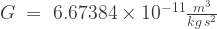
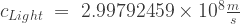


 ) body, of the “collective” net mass system body; which includes its “Self” attraction and interaction force.
 ) distance, relative to the center of the Gradient Gravitational Field.


 ); and likewise varies in direct proportion to the square of the
  ), and varies inversely with the square of the


 ) describes the acceleration of mass and energy, towards the center of the gradient gravity field, and towards ever decreasing and smaller volumes of spherical gradient shell potentials.


 )
)  )
) 


 ) is the measure of the work done by the
  ), relative to the center of the gradient gravity field.
![{dV_{Gravity-Potential}}\,\,=\,\,(-)\vec{F_{Gravity}}\,\vec{dr}\,\,=\,\,(+)[\frac{m_{mass}\,m_{Net}\,G}{r^2}]\,{dr}](https://s0.wp.com/latex.php?latex=%7BdV_%7BGravity-Potential%7D%7D%5C%2C%5C%2C%3D%5C%2C%5C%2C%28-%29%5Cvec%7BF_%7BGravity%7D%7D%5C%2C%5Cvec%7Bdr%7D%5C%2C%5C%2C%3D%5C%2C%5C%2C%28%2B%29%5B%5Cfrac%7Bm_%7Bmass%7D%5C%2Cm_%7BNet%7D%5C%2CG%7D%7Br%5E2%7D%5D%5C%2C%7Bdr%7D&bg=ffffff&fg=333333&s=1&c=20201002)


 ) distance, relative to the center of the Gradient Gravitational Field.

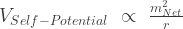


 ) is a measure of the square of the orbiting/spin/rotation squared tangential velocity of each potential of the gradient gravity field; and describes the squared velocity “inertia” potential, of the relative spatial separation, of the attraction and interaction of “mass towards mass”; and towards the center of the gradient gravity field, and towards ever decreasing and smaller volumes, of spherical gradient shell potentials.
 ); and likewise varies in direct proportion to the

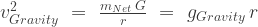


 ) of the the gradient field, dependent only on the inverse distance from the center of the field.
 ) distance is to the “mean center” and
  ) Black Hole Event Horizon of the system.
 ) distance is from the “mean center” and the
  ) constant, at the core of the gradient field, and its
  ) distance is equal to the
  ) distance is equal to infinity, or an infinite distance away from the “mean center” of the gradient gravity field system body.
 ) of each concentric spherical shell potential of the gradient gravity field.


 ), and changes as a function of the “Euclidean Radius” (
 ) of a symmetric sphere, as derived in Section 3, of the work:


 ) – in the


 ) – in the


 ) – in the


 ) – in the
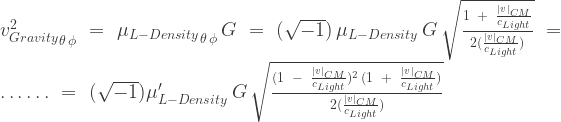


 ) – in the
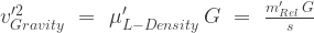
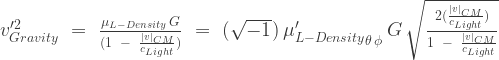


 ) – in the
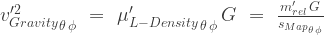


![\vec{F_{Self-Gravity}}\,\,=\,\,(-){\mu'^2_{L-Density}\,G}\,{({1\;\;-\;\;\frac{|v|_{CM}}{c_{Light}}})^2}\,\hat{a}_{r}\,\,=\,\,{\mu^2_{L-Density}}_{\theta \, \phi}\,[{\frac{2(\frac{|v|_{CM}}{c_{Light}})}{1\;\;+\;\;\frac{|v|_{CM}}{c_{Light}}}}]\,\,\hat{a}_{r}](https://s0.wp.com/latex.php?latex=%5Cvec%7BF_%7BSelf-Gravity%7D%7D%5C%2C%5C%2C%3D%5C%2C%5C%2C%28-%29%7B%5Cmu%27%5E2_%7BL-Density%7D%5C%2CG%7D%5C%2C%7B%28%7B1%5C%3B%5C%3B-%5C%3B%5C%3B%5Cfrac%7B%7Cv%7C_%7BCM%7D%7D%7Bc_%7BLight%7D%7D%7D%29%5E2%7D%5C%2C%5Chat%7Ba%7D_%7Br%7D%5C%2C%5C%2C%3D%5C%2C%5C%2C%7B%5Cmu%5E2_%7BL-Density%7D%7D_%7B%5Ctheta+%5C%2C+%5Cphi%7D%5C%2C%5B%7B%5Cfrac%7B2%28%5Cfrac%7B%7Cv%7C_%7BCM%7D%7D%7Bc_%7BLight%7D%7D%29%7D%7B1%5C%3B%5C%3B%2B%5C%3B%5C%3B%5Cfrac%7B%7Cv%7C_%7BCM%7D%7D%7Bc_%7BLight%7D%7D%7D%7D%5D%5C%2C%5C%2C%5Chat%7Ba%7D_%7Br%7D&bg=ffffff&fg=333333&s=1&c=20201002)
![\vec{F_{Self-Gravity}}\,=\,(-)\frac{m^2_{Net}\,G}{r^2}\,\,\hat{a}_{r}\,=\,(\frac{m'^2_{Rel}\,G}{s^2}){({1\;\;-\;\;\frac{|v|_{CM}}{c_{Light}}})^2}\,\,\hat{a}_{r}\,=\,(\frac{m^2_{Net}\,G}{{s^2_{Map}}_{\theta \, \phi}})\,[{\frac{2(\frac{|v|_{CM}}{c_{Light}})}{1\;\;+\;\;\frac{|v|_{CM}}{c_{Light}}}}]\,\,\hat{a}_{r}](https://s0.wp.com/latex.php?latex=%5Cvec%7BF_%7BSelf-Gravity%7D%7D%5C%2C%3D%5C%2C%28-%29%5Cfrac%7Bm%5E2_%7BNet%7D%5C%2CG%7D%7Br%5E2%7D%5C%2C%5C%2C%5Chat%7Ba%7D_%7Br%7D%5C%2C%3D%5C%2C%28%5Cfrac%7Bm%27%5E2_%7BRel%7D%5C%2CG%7D%7Bs%5E2%7D%29%7B%28%7B1%5C%3B%5C%3B-%5C%3B%5C%3B%5Cfrac%7B%7Cv%7C_%7BCM%7D%7D%7Bc_%7BLight%7D%7D%7D%29%5E2%7D%5C%2C%5C%2C%5Chat%7Ba%7D_%7Br%7D%5C%2C%3D%5C%2C%28%5Cfrac%7Bm%5E2_%7BNet%7D%5C%2CG%7D%7B%7Bs%5E2_%7BMap%7D%7D_%7B%5Ctheta+%5C%2C+%5Cphi%7D%7D%29%5C%2C%5B%7B%5Cfrac%7B2%28%5Cfrac%7B%7Cv%7C_%7BCM%7D%7D%7Bc_%7BLight%7D%7D%29%7D%7B1%5C%3B%5C%3B%2B%5C%3B%5C%3B%5Cfrac%7B%7Cv%7C_%7BCM%7D%7D%7Bc_%7BLight%7D%7D%7D%7D%5D%5C%2C%5C%2C%5Chat%7Ba%7D_%7Br%7D&bg=ffffff&fg=333333&s=1&c=20201002)
![\vec{F_{Self-Gravity}}_{\theta \, \phi}\,\,=\,\,(-){\mu^2_{L-Density}}_{\theta \, \phi}\,{G}\,\,\hat{a}_{r}\,\,=\,\,{\mu^2_{L-Density}}\,{G}\,[{\frac{1\;\;+\;\;\frac{|v|_{CM}}{c_{Light}}}{2(\frac{|v|_{CM}}{c_{Light}})}}]\,\,\hat{a}_{r}\,\,=\,\,\dots\dots\,\,=\,\,{\mu'^2_{L-Density}}\,{G}\,[{\frac{(1\;\;-\;\;\frac{|v|_{CM}}{c_{Light}})^2\,(1\;\;+\;\;\frac{|v|_{CM}}{c_{Light}})}{2(\frac{|v|_{CM}}{c_{Light}})}}]\,\,\hat{a}_{r}](https://s0.wp.com/latex.php?latex=%5Cvec%7BF_%7BSelf-Gravity%7D%7D_%7B%5Ctheta+%5C%2C+%5Cphi%7D%5C%2C%5C%2C%3D%5C%2C%5C%2C%28-%29%7B%5Cmu%5E2_%7BL-Density%7D%7D_%7B%5Ctheta+%5C%2C+%5Cphi%7D%5C%2C%7BG%7D%5C%2C%5C%2C%5Chat%7Ba%7D_%7Br%7D%5C%2C%5C%2C%3D%5C%2C%5C%2C%7B%5Cmu%5E2_%7BL-Density%7D%7D%5C%2C%7BG%7D%5C%2C%5B%7B%5Cfrac%7B1%5C%3B%5C%3B%2B%5C%3B%5C%3B%5Cfrac%7B%7Cv%7C_%7BCM%7D%7D%7Bc_%7BLight%7D%7D%7D%7B2%28%5Cfrac%7B%7Cv%7C_%7BCM%7D%7D%7Bc_%7BLight%7D%7D%29%7D%7D%5D%5C%2C%5C%2C%5Chat%7Ba%7D_%7Br%7D%5C%2C%5C%2C%3D%5C%2C%5C%2C%5Cdots%5Cdots%5C%2C%5C%2C%3D%5C%2C%5C%2C%7B%5Cmu%27%5E2_%7BL-Density%7D%7D%5C%2C%7BG%7D%5C%2C%5B%7B%5Cfrac%7B%281%5C%3B%5C%3B-%5C%3B%5C%3B%5Cfrac%7B%7Cv%7C_%7BCM%7D%7D%7Bc_%7BLight%7D%7D%29%5E2%5C%2C%281%5C%3B%5C%3B%2B%5C%3B%5C%3B%5Cfrac%7B%7Cv%7C_%7BCM%7D%7D%7Bc_%7BLight%7D%7D%29%7D%7B2%28%5Cfrac%7B%7Cv%7C_%7BCM%7D%7D%7Bc_%7BLight%7D%7D%29%7D%7D%5D%5C%2C%5C%2C%5Chat%7Ba%7D_%7Br%7D&bg=ffffff&fg=333333&s=1&c=20201002)
![\vec{F_{Self-Gravity}}_{\theta \, \phi}\,\,=\,\,(\frac{m^2_{Net}\,G}{r^2})\,[{\frac{1\;\;+\;\;\frac{|v|_{CM}}{c_{Light}}}{2(\frac{|v|_{CM}}{c_{Light}})}}]\,\,\hat{a}_{r}\,\,=\,\,(\frac{m'^2_{Rel}\,G}{s^2})\,[{\frac{(1\;\;-\;\;\frac{|v|_{CM}}{c_{Light}})^2\,(1\;\;+\;\;\frac{|v|_{CM}}{c_{Light}})}{2(\frac{|v|_{CM}}{c_{Light}})}}]\,\,\hat{a}_{r}](https://s0.wp.com/latex.php?latex=%5Cvec%7BF_%7BSelf-Gravity%7D%7D_%7B%5Ctheta+%5C%2C+%5Cphi%7D%5C%2C%5C%2C%3D%5C%2C%5C%2C%28%5Cfrac%7Bm%5E2_%7BNet%7D%5C%2CG%7D%7Br%5E2%7D%29%5C%2C%5B%7B%5Cfrac%7B1%5C%3B%5C%3B%2B%5C%3B%5C%3B%5Cfrac%7B%7Cv%7C_%7BCM%7D%7D%7Bc_%7BLight%7D%7D%7D%7B2%28%5Cfrac%7B%7Cv%7C_%7BCM%7D%7D%7Bc_%7BLight%7D%7D%29%7D%7D%5D%5C%2C%5C%2C%5Chat%7Ba%7D_%7Br%7D%5C%2C%5C%2C%3D%5C%2C%5C%2C%28%5Cfrac%7Bm%27%5E2_%7BRel%7D%5C%2CG%7D%7Bs%5E2%7D%29%5C%2C%5B%7B%5Cfrac%7B%281%5C%3B%5C%3B-%5C%3B%5C%3B%5Cfrac%7B%7Cv%7C_%7BCM%7D%7D%7Bc_%7BLight%7D%7D%29%5E2%5C%2C%281%5C%3B%5C%3B%2B%5C%3B%5C%3B%5Cfrac%7B%7Cv%7C_%7BCM%7D%7D%7Bc_%7BLight%7D%7D%29%7D%7B2%28%5Cfrac%7B%7Cv%7C_%7BCM%7D%7D%7Bc_%7BLight%7D%7D%29%7D%7D%5D%5C%2C%5C%2C%5Chat%7Ba%7D_%7Br%7D&bg=ffffff&fg=333333&s=1&c=20201002)
![\vec{F'_{Self-Gravity}}\,\,=\,\,(-)\frac{{\mu^2_{L-Density}}\,G}{({1\;\;-\;\;\frac{|v|_{CM}}{c_{Light}}})^2}\,\,\hat{a}_{r}\,\,=\,\,{\mu'^2_{L-Density}}_{\theta \, \phi}\,{G}\,[{\frac{2(\frac{|v|_{CM}}{c_{Light}})}{1\;\;-\;\;\frac{|v|_{CM}}{c_{Light}}}}]\,\,\hat{a}_{r}](https://s0.wp.com/latex.php?latex=%5Cvec%7BF%27_%7BSelf-Gravity%7D%7D%5C%2C%5C%2C%3D%5C%2C%5C%2C%28-%29%5Cfrac%7B%7B%5Cmu%5E2_%7BL-Density%7D%7D%5C%2CG%7D%7B%28%7B1%5C%3B%5C%3B-%5C%3B%5C%3B%5Cfrac%7B%7Cv%7C_%7BCM%7D%7D%7Bc_%7BLight%7D%7D%7D%29%5E2%7D%5C%2C%5C%2C%5Chat%7Ba%7D_%7Br%7D%5C%2C%5C%2C%3D%5C%2C%5C%2C%7B%5Cmu%27%5E2_%7BL-Density%7D%7D_%7B%5Ctheta+%5C%2C+%5Cphi%7D%5C%2C%7BG%7D%5C%2C%5B%7B%5Cfrac%7B2%28%5Cfrac%7B%7Cv%7C_%7BCM%7D%7D%7Bc_%7BLight%7D%7D%29%7D%7B1%5C%3B%5C%3B-%5C%3B%5C%3B%5Cfrac%7B%7Cv%7C_%7BCM%7D%7D%7Bc_%7BLight%7D%7D%7D%7D%5D%5C%2C%5C%2C%5Chat%7Ba%7D_%7Br%7D&bg=ffffff&fg=333333&s=1&c=20201002)
![\vec{F'_{Self-Gravity}}\,=\,(-)\frac{m'^2_{Rel}\,G}{s^2}\,\hat{a}_{r}\,=\,(-)\frac{m^2_{Net}\,G}{r^2}{({1\,-\,\frac{|v|_{CM}}{c_{Light}}})^{-2}}\,\hat{a}_{r}\,=\,(\frac{m'^2_{Rel}\,G}{{s^2_{Map}}_{\theta \, \phi}})\,[{\frac{2(\frac{|v|_{CM}}{c_{Light}})}{1\,-\,\frac{|v|_{CM}}{c_{Light}}}}]\,\hat{a}_{r}](https://s0.wp.com/latex.php?latex=%5Cvec%7BF%27_%7BSelf-Gravity%7D%7D%5C%2C%3D%5C%2C%28-%29%5Cfrac%7Bm%27%5E2_%7BRel%7D%5C%2CG%7D%7Bs%5E2%7D%5C%2C%5Chat%7Ba%7D_%7Br%7D%5C%2C%3D%5C%2C%28-%29%5Cfrac%7Bm%5E2_%7BNet%7D%5C%2CG%7D%7Br%5E2%7D%7B%28%7B1%5C%2C-%5C%2C%5Cfrac%7B%7Cv%7C_%7BCM%7D%7D%7Bc_%7BLight%7D%7D%7D%29%5E%7B-2%7D%7D%5C%2C%5Chat%7Ba%7D_%7Br%7D%5C%2C%3D%5C%2C%28%5Cfrac%7Bm%27%5E2_%7BRel%7D%5C%2CG%7D%7B%7Bs%5E2_%7BMap%7D%7D_%7B%5Ctheta+%5C%2C+%5Cphi%7D%7D%29%5C%2C%5B%7B%5Cfrac%7B2%28%5Cfrac%7B%7Cv%7C_%7BCM%7D%7D%7Bc_%7BLight%7D%7D%29%7D%7B1%5C%2C-%5C%2C%5Cfrac%7B%7Cv%7C_%7BCM%7D%7D%7Bc_%7BLight%7D%7D%7D%7D%5D%5C%2C%5Chat%7Ba%7D_%7Br%7D&bg=ffffff&fg=333333&s=1&c=20201002)
![\vec{F'_{Self-Gravity}}_{\theta \, \phi}\,\,=\,\,{\mu'^2_{L-Density}}\,{G}\,[{\frac{1\;\;-\;\;\frac{|v|_{CM}}{c_{Light}}}{2(\frac{|v|_{CM}}{c_{Light}})}}]\,\,\hat{a}_{r}\,\,=\,\,{\mu^2_{L-Density}}\,{G}\,[{\frac{1}{2(\frac{|v|_{CM}}{c_{Light}})\,(1\;\;-\;\;\frac{|v|_{CM}}{c_{Light}})}}]\,\,\hat{a}_{r}](https://s0.wp.com/latex.php?latex=%5Cvec%7BF%27_%7BSelf-Gravity%7D%7D_%7B%5Ctheta+%5C%2C+%5Cphi%7D%5C%2C%5C%2C%3D%5C%2C%5C%2C%7B%5Cmu%27%5E2_%7BL-Density%7D%7D%5C%2C%7BG%7D%5C%2C%5B%7B%5Cfrac%7B1%5C%3B%5C%3B-%5C%3B%5C%3B%5Cfrac%7B%7Cv%7C_%7BCM%7D%7D%7Bc_%7BLight%7D%7D%7D%7B2%28%5Cfrac%7B%7Cv%7C_%7BCM%7D%7D%7Bc_%7BLight%7D%7D%29%7D%7D%5D%5C%2C%5C%2C%5Chat%7Ba%7D_%7Br%7D%5C%2C%5C%2C%3D%5C%2C%5C%2C%7B%5Cmu%5E2_%7BL-Density%7D%7D%5C%2C%7BG%7D%5C%2C%5B%7B%5Cfrac%7B1%7D%7B2%28%5Cfrac%7B%7Cv%7C_%7BCM%7D%7D%7Bc_%7BLight%7D%7D%29%5C%2C%281%5C%3B%5C%3B-%5C%3B%5C%3B%5Cfrac%7B%7Cv%7C_%7BCM%7D%7D%7Bc_%7BLight%7D%7D%29%7D%7D%5D%5C%2C%5C%2C%5Chat%7Ba%7D_%7Br%7D&bg=ffffff&fg=333333&s=1&c=20201002)
![\vec{F'_{Self-Gravity}}_{\theta \, \phi}\,\,=\,\,(\frac{m'^2_{Rel}\,G}{s^2})\,[{\frac{1\;\;-\;\;\frac{|v|_{CM}}{c_{Light}}}{2(\frac{|v|_{CM}}{c_{Light}})}}]\,\hat{a}_{r}\,\,=\,\,(\frac{m^2_{Net}\,G}{r^2})\,[{\frac{1}{2(\frac{|v|_{CM}}{c_{Light}})\,(1\;\;-\;\;\frac{|v|_{CM}}{c_{Light}})}}]\,\hat{a}_{r}](https://s0.wp.com/latex.php?latex=%5Cvec%7BF%27_%7BSelf-Gravity%7D%7D_%7B%5Ctheta+%5C%2C+%5Cphi%7D%5C%2C%5C%2C%3D%5C%2C%5C%2C%28%5Cfrac%7Bm%27%5E2_%7BRel%7D%5C%2CG%7D%7Bs%5E2%7D%29%5C%2C%5B%7B%5Cfrac%7B1%5C%3B%5C%3B-%5C%3B%5C%3B%5Cfrac%7B%7Cv%7C_%7BCM%7D%7D%7Bc_%7BLight%7D%7D%7D%7B2%28%5Cfrac%7B%7Cv%7C_%7BCM%7D%7D%7Bc_%7BLight%7D%7D%29%7D%7D%5D%5C%2C%5Chat%7Ba%7D_%7Br%7D%5C%2C%5C%2C%3D%5C%2C%5C%2C%28%5Cfrac%7Bm%5E2_%7BNet%7D%5C%2CG%7D%7Br%5E2%7D%29%5C%2C%5B%7B%5Cfrac%7B1%7D%7B2%28%5Cfrac%7B%7Cv%7C_%7BCM%7D%7D%7Bc_%7BLight%7D%7D%29%5C%2C%281%5C%3B%5C%3B-%5C%3B%5C%3B%5Cfrac%7B%7Cv%7C_%7BCM%7D%7D%7Bc_%7BLight%7D%7D%29%7D%7D%5D%5C%2C%5Chat%7Ba%7D_%7Br%7D&bg=ffffff&fg=333333&s=1&c=20201002)

 ) will be described below. Limiting, the discussion to the
 ![{g_{Gravity}}\;\;=\;\;(-)({m_{Net}\,G})\,[\frac{1 \;\;+\;\;\frac{|v|_{CM}}{c_{Light}}}{2(\frac{|v|_{CM}}{c_{Light}})}]\,\frac{\vec{d\Omega^2_{Map}}_{(\theta \phi)}}{dr^2}](https://s0.wp.com/latex.php?latex=%7Bg_%7BGravity%7D%7D%5C%3B%5C%3B%3D%5C%3B%5C%3B%28-%29%28%7Bm_%7BNet%7D%5C%2CG%7D%29%5C%2C%5B%5Cfrac%7B1+%5C%3B%5C%3B%2B%5C%3B%5C%3B%5Cfrac%7B%7Cv%7C_%7BCM%7D%7D%7Bc_%7BLight%7D%7D%7D%7B2%28%5Cfrac%7B%7Cv%7C_%7BCM%7D%7D%7Bc_%7BLight%7D%7D%29%7D%5D%5C%2C%5Cfrac%7B%5Cvec%7Bd%5COmega%5E2_%7BMap%7D%7D_%7B%28%5Ctheta+%5Cphi%29%7D%7D%7Bdr%5E2%7D&bg=ffffff&fg=333333&s=1&c=20201002)
![{g_{Gravity}}\;\;=\;\;(-)(\frac{m_{Net}\,G}{c^2_{Light}})\,[\frac{1 \;\;+\;\;\frac{|v|_{CM}}{c_{Light}}}{2(\frac{|v|_{CM}}{c_{Light}})}]\,\frac{\vec{d\Omega^2_{Map}}_{(\theta \phi)}}{dt^2_{Light}}](https://s0.wp.com/latex.php?latex=%7Bg_%7BGravity%7D%7D%5C%3B%5C%3B%3D%5C%3B%5C%3B%28-%29%28%5Cfrac%7Bm_%7BNet%7D%5C%2CG%7D%7Bc%5E2_%7BLight%7D%7D%29%5C%2C%5B%5Cfrac%7B1+%5C%3B%5C%3B%2B%5C%3B%5C%3B%5Cfrac%7B%7Cv%7C_%7BCM%7D%7D%7Bc_%7BLight%7D%7D%7D%7B2%28%5Cfrac%7B%7Cv%7C_%7BCM%7D%7D%7Bc_%7BLight%7D%7D%29%7D%5D%5C%2C%5Cfrac%7B%5Cvec%7Bd%5COmega%5E2_%7BMap%7D%7D_%7B%28%5Ctheta+%5Cphi%29%7D%7D%7Bdt%5E2_%7BLight%7D%7D&bg=ffffff&fg=333333&s=1&c=20201002)
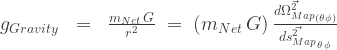

 ) Space & Time Metric and in the
 ![{g_{Gravity}}\;\;=\;\;(-)({m'_{Rel}\,G})\,[\frac{\sqrt{(1 \;\;-\;\;\frac{|v|_{CM}}{c_{Light}})^3\,(1 \;\;+\;\;\frac{|v|_{CM}}{c_{Light}})}}{2(\frac{|v|_{CM}}{c_{Light}})}]\,\frac{\vec{d\Omega^2_{Map}}_{(\theta \phi)}}{ds^2}](https://s0.wp.com/latex.php?latex=%7Bg_%7BGravity%7D%7D%5C%3B%5C%3B%3D%5C%3B%5C%3B%28-%29%28%7Bm%27_%7BRel%7D%5C%2CG%7D%29%5C%2C%5B%5Cfrac%7B%5Csqrt%7B%281+%5C%3B%5C%3B-%5C%3B%5C%3B%5Cfrac%7B%7Cv%7C_%7BCM%7D%7D%7Bc_%7BLight%7D%7D%29%5E3%5C%2C%281+%5C%3B%5C%3B%2B%5C%3B%5C%3B%5Cfrac%7B%7Cv%7C_%7BCM%7D%7D%7Bc_%7BLight%7D%7D%29%7D%7D%7B2%28%5Cfrac%7B%7Cv%7C_%7BCM%7D%7D%7Bc_%7BLight%7D%7D%29%7D%5D%5C%2C%5Cfrac%7B%5Cvec%7Bd%5COmega%5E2_%7BMap%7D%7D_%7B%28%5Ctheta+%5Cphi%29%7D%7D%7Bds%5E2%7D&bg=ffffff&fg=333333&s=1&c=20201002)
![{g_{Gravity}}\;\;=\;\;(-)(\frac{m'_{Rel}\,G}{c^2_{Light}})\,[\frac{\sqrt{(1 \;\;-\;\;\frac{|v|_{CM}}{c_{Light}})^3\,(1 \;\;+\;\;\frac{|v|_{CM}}{c_{Light}})}}{2(\frac{|v|_{CM}}{c_{Light}})}]\,\frac{\vec{d\Omega^2_{Map}}_{(\theta \phi)}}{dt'^2_{Light(s)}}](https://s0.wp.com/latex.php?latex=%7Bg_%7BGravity%7D%7D%5C%3B%5C%3B%3D%5C%3B%5C%3B%28-%29%28%5Cfrac%7Bm%27_%7BRel%7D%5C%2CG%7D%7Bc%5E2_%7BLight%7D%7D%29%5C%2C%5B%5Cfrac%7B%5Csqrt%7B%281+%5C%3B%5C%3B-%5C%3B%5C%3B%5Cfrac%7B%7Cv%7C_%7BCM%7D%7D%7Bc_%7BLight%7D%7D%29%5E3%5C%2C%281+%5C%3B%5C%3B%2B%5C%3B%5C%3B%5Cfrac%7B%7Cv%7C_%7BCM%7D%7D%7Bc_%7BLight%7D%7D%29%7D%7D%7B2%28%5Cfrac%7B%7Cv%7C_%7BCM%7D%7D%7Bc_%7BLight%7D%7D%29%7D%5D%5C%2C%5Cfrac%7B%5Cvec%7Bd%5COmega%5E2_%7BMap%7D%7D_%7B%28%5Ctheta+%5Cphi%29%7D%7D%7Bdt%27%5E2_%7BLight%28s%29%7D%7D&bg=ffffff&fg=333333&s=1&c=20201002)

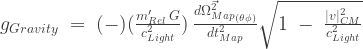


 ) Cartesian Coordinates
![\vec{dr^2}\;=\;\vec{c^2_{Light}}\,{dt^2_{Light}}\;=\; [\vec{dx^2}\;+\;\vec{dy^2}\;+\;\vec{dz^2}]](https://s0.wp.com/latex.php?latex=%5Cvec%7Bdr%5E2%7D%5C%3B%3D%5C%3B%5Cvec%7Bc%5E2_%7BLight%7D%7D%5C%2C%7Bdt%5E2_%7BLight%7D%7D%5C%3B%3D%5C%3B+%5B%5Cvec%7Bdx%5E2%7D%5C%3B%2B%5C%3B%5Cvec%7Bdy%5E2%7D%5C%3B%2B%5C%3B%5Cvec%7Bdz%5E2%7D%5D&bg=ffffff&fg=333333&s=1&c=20201002)

![\vec{dr^2}\;=\; [\vec{ds^2}\;-\;\vec{ds^2_{Map}}_{\theta \, \phi}]\;=\; [\vec{dx^2}\;+\;\vec{dy^2}\;+\;\vec{dz^2}]](https://s0.wp.com/latex.php?latex=%5Cvec%7Bdr%5E2%7D%5C%3B%3D%5C%3B+%5B%5Cvec%7Bds%5E2%7D%5C%3B-%5C%3B%5Cvec%7Bds%5E2_%7BMap%7D%7D_%7B%5Ctheta+%5C%2C+%5Cphi%7D%5D%5C%3B%3D%5C%3B+%5B%5Cvec%7Bdx%5E2%7D%5C%3B%2B%5C%3B%5Cvec%7Bdy%5E2%7D%5C%3B%2B%5C%3B%5Cvec%7Bdz%5E2%7D%5D&bg=ffffff&fg=333333&s=1&c=20201002)
![\vec{dr^2}\;=\;\vec{c^2_{Light}}\,{dt^2_{Light}}\;=\; [\vec{c^2_{Light}}\,{dt'^2_{Light(s)}}\;+\;\vec{c^2_{Light}}\,{dt^2_{Map}}]](https://s0.wp.com/latex.php?latex=%5Cvec%7Bdr%5E2%7D%5C%3B%3D%5C%3B%5Cvec%7Bc%5E2_%7BLight%7D%7D%5C%2C%7Bdt%5E2_%7BLight%7D%7D%5C%3B%3D%5C%3B+%5B%5Cvec%7Bc%5E2_%7BLight%7D%7D%5C%2C%7Bdt%27%5E2_%7BLight%28s%29%7D%7D%5C%3B%2B%5C%3B%5Cvec%7Bc%5E2_%7BLight%7D%7D%5C%2C%7Bdt%5E2_%7BMap%7D%7D%5D&bg=ffffff&fg=333333&s=1&c=20201002)

 ) “Geodesic” Metric, relative to the
 ![\vec{dr^2}\;=\;\vec{ds^2}[\frac{1 \;\;+\;\;\frac{|v|_{CM}}{c_{Light}}}{1 \;\;-\;\;\frac{|v|_{CM}}{c_{Light}}}]\;\;=\;\;{(-){\vec{ds^2_{Map}}_{\theta \, \phi}}}[\frac{1 \;\;+\;\;\frac{|v|_{CM}}{c_{Light}}}{2(\frac{|v|_{CM}}{c_{Light}})}]\;](https://s0.wp.com/latex.php?latex=%5Cvec%7Bdr%5E2%7D%5C%3B%3D%5C%3B%5Cvec%7Bds%5E2%7D%5B%5Cfrac%7B1+%5C%3B%5C%3B%2B%5C%3B%5C%3B%5Cfrac%7B%7Cv%7C_%7BCM%7D%7D%7Bc_%7BLight%7D%7D%7D%7B1+%5C%3B%5C%3B-%5C%3B%5C%3B%5Cfrac%7B%7Cv%7C_%7BCM%7D%7D%7Bc_%7BLight%7D%7D%7D%5D%5C%3B%5C%3B%3D%5C%3B%5C%3B%7B%28-%29%7B%5Cvec%7Bds%5E2_%7BMap%7D%7D_%7B%5Ctheta+%5C%2C+%5Cphi%7D%7D%7D%5B%5Cfrac%7B1+%5C%3B%5C%3B%2B%5C%3B%5C%3B%5Cfrac%7B%7Cv%7C_%7BCM%7D%7D%7Bc_%7BLight%7D%7D%7D%7B2%28%5Cfrac%7B%7Cv%7C_%7BCM%7D%7D%7Bc_%7BLight%7D%7D%29%7D%5D%5C%3B&bg=ffffff&fg=333333&s=1&c=20201002)

![\vec{dr^2}\;=\;\frac{3\,\vec{ds^2}\;\;-\;\;[\frac{(1 \;\;-\;\;\frac{|v|_{CM}}{c_{Light}})}{2(\frac{c_{Light}}{|v|_{CM}})}]\,\vec{ds^2_{Map}}_{\theta \, \phi}}{(1 \;\;-\;\;\frac{|v|^2_{CM}}{c^2_{Light}})}\;=\;\frac{3\,\vec{ds^2}\;\;+\;\;[\frac{(1 \;\;-\;\;\frac{|v|_{CM}}{c_{Light}})}{2(\frac{c_{Light}}{|v|_{CM}})}]\,\vec{c^2_{Light}}\,{dt^2_{Map}}}{(1 \;\;-\;\;\frac{|v|^2_{CM}}{c^2_{Light}})}](https://s0.wp.com/latex.php?latex=%5Cvec%7Bdr%5E2%7D%5C%3B%3D%5C%3B%5Cfrac%7B3%5C%2C%5Cvec%7Bds%5E2%7D%5C%3B%5C%3B-%5C%3B%5C%3B%5B%5Cfrac%7B%281+%5C%3B%5C%3B-%5C%3B%5C%3B%5Cfrac%7B%7Cv%7C_%7BCM%7D%7D%7Bc_%7BLight%7D%7D%29%7D%7B2%28%5Cfrac%7Bc_%7BLight%7D%7D%7B%7Cv%7C_%7BCM%7D%7D%29%7D%5D%5C%2C%5Cvec%7Bds%5E2_%7BMap%7D%7D_%7B%5Ctheta+%5C%2C+%5Cphi%7D%7D%7B%281+%5C%3B%5C%3B-%5C%3B%5C%3B%5Cfrac%7B%7Cv%7C%5E2_%7BCM%7D%7D%7Bc%5E2_%7BLight%7D%7D%29%7D%5C%3B%3D%5C%3B%5Cfrac%7B3%5C%2C%5Cvec%7Bds%5E2%7D%5C%3B%5C%3B%2B%5C%3B%5C%3B%5B%5Cfrac%7B%281+%5C%3B%5C%3B-%5C%3B%5C%3B%5Cfrac%7B%7Cv%7C_%7BCM%7D%7D%7Bc_%7BLight%7D%7D%29%7D%7B2%28%5Cfrac%7Bc_%7BLight%7D%7D%7B%7Cv%7C_%7BCM%7D%7D%29%7D%5D%5C%2C%5Cvec%7Bc%5E2_%7BLight%7D%7D%5C%2C%7Bdt%5E2_%7BMap%7D%7D%7D%7B%281+%5C%3B%5C%3B-%5C%3B%5C%3B%5Cfrac%7B%7Cv%7C%5E2_%7BCM%7D%7D%7Bc%5E2_%7BLight%7D%7D%29%7D&bg=ffffff&fg=333333&s=1&c=20201002)


![{dt^2_{Light}}\;=\;[{dt'^2_{Light(s)}}\;\;+\;\;{dt^2_{Map}}]\;=\;[{dt'^2_{Light(s)}}\;\;-\;\;\frac{(\vec{ds^2_{Map}}_{\theta \, \phi})^2}{c^2_{Light}}]](https://s0.wp.com/latex.php?latex=%7Bdt%5E2_%7BLight%7D%7D%5C%3B%3D%5C%3B%5B%7Bdt%27%5E2_%7BLight%28s%29%7D%7D%5C%3B%5C%3B%2B%5C%3B%5C%3B%7Bdt%5E2_%7BMap%7D%7D%5D%5C%3B%3D%5C%3B%5B%7Bdt%27%5E2_%7BLight%28s%29%7D%7D%5C%3B%5C%3B-%5C%3B%5C%3B%5Cfrac%7B%28%5Cvec%7Bds%5E2_%7BMap%7D%7D_%7B%5Ctheta+%5C%2C+%5Cphi%7D%29%5E2%7D%7Bc%5E2_%7BLight%7D%7D%5D&bg=ffffff&fg=333333&s=1&c=20201002)
 ) – measured in the
  ), relative to the
  ), relative to the
 ![{dt^2_{Light}}\;=\;{dt'^2_{Light(s)}}[\frac{1 \;\;+\;\;\frac{|v|_{CM}}{c_{Light}}}{1 \;\;-\;\;\frac{|v|_{CM}}{c_{Light}}}]\;\;=\;\;{dt^2_{Map}}[\frac{1 \;\;+\;\;\frac{|v|_{CM}}{c_{Light}}}{2(\frac{|v|_{CM}}{c_{Light}})}]\;](https://s0.wp.com/latex.php?latex=%7Bdt%5E2_%7BLight%7D%7D%5C%3B%3D%5C%3B%7Bdt%27%5E2_%7BLight%28s%29%7D%7D%5B%5Cfrac%7B1+%5C%3B%5C%3B%2B%5C%3B%5C%3B%5Cfrac%7B%7Cv%7C_%7BCM%7D%7D%7Bc_%7BLight%7D%7D%7D%7B1+%5C%3B%5C%3B-%5C%3B%5C%3B%5Cfrac%7B%7Cv%7C_%7BCM%7D%7D%7Bc_%7BLight%7D%7D%7D%5D%5C%3B%5C%3B%3D%5C%3B%5C%3B%7Bdt%5E2_%7BMap%7D%7D%5B%5Cfrac%7B1+%5C%3B%5C%3B%2B%5C%3B%5C%3B%5Cfrac%7B%7Cv%7C_%7BCM%7D%7D%7Bc_%7BLight%7D%7D%7D%7B2%28%5Cfrac%7B%7Cv%7C_%7BCM%7D%7D%7Bc_%7BLight%7D%7D%29%7D%5D%5C%3B&bg=ffffff&fg=333333&s=1&c=20201002)

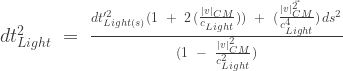
![{dt^2_{Light}}\;=\;\frac{3\,{dt'^2_{Light(s)}}\;\;-\;\;(\frac{1}{c^2_{Light}})[\frac{(1 \;\;-\;\;\frac{|v|_{CM}}{c_{Light}})}{2(\frac{c_{Light}}{|v|_{CM}})}]\,\vec{ds^2_{Map}}_{\theta \, \phi}}{(1 \;\;-\;\;\frac{|v|^2_{CM}}{c^2_{Light}})}\;=\;\frac{3\,{dt'^2_{Light(s)}}\;\;+\;\;[\frac{(1 \;\;-\;\;\frac{|v|_{CM}}{c_{Light}})}{2(\frac{c_{Light}}{|v|_{CM}})}]\,{dt^2_{Map}}}{(1 \;\;-\;\;\frac{|v|^2_{CM}}{c^2_{Light}})}](https://s0.wp.com/latex.php?latex=%7Bdt%5E2_%7BLight%7D%7D%5C%3B%3D%5C%3B%5Cfrac%7B3%5C%2C%7Bdt%27%5E2_%7BLight%28s%29%7D%7D%5C%3B%5C%3B-%5C%3B%5C%3B%28%5Cfrac%7B1%7D%7Bc%5E2_%7BLight%7D%7D%29%5B%5Cfrac%7B%281+%5C%3B%5C%3B-%5C%3B%5C%3B%5Cfrac%7B%7Cv%7C_%7BCM%7D%7D%7Bc_%7BLight%7D%7D%29%7D%7B2%28%5Cfrac%7Bc_%7BLight%7D%7D%7B%7Cv%7C_%7BCM%7D%7D%29%7D%5D%5C%2C%5Cvec%7Bds%5E2_%7BMap%7D%7D_%7B%5Ctheta+%5C%2C+%5Cphi%7D%7D%7B%281+%5C%3B%5C%3B-%5C%3B%5C%3B%5Cfrac%7B%7Cv%7C%5E2_%7BCM%7D%7D%7Bc%5E2_%7BLight%7D%7D%29%7D%5C%3B%3D%5C%3B%5Cfrac%7B3%5C%2C%7Bdt%27%5E2_%7BLight%28s%29%7D%7D%5C%3B%5C%3B%2B%5C%3B%5C%3B%5B%5Cfrac%7B%281+%5C%3B%5C%3B-%5C%3B%5C%3B%5Cfrac%7B%7Cv%7C_%7BCM%7D%7D%7Bc_%7BLight%7D%7D%29%7D%7B2%28%5Cfrac%7Bc_%7BLight%7D%7D%7B%7Cv%7C_%7BCM%7D%7D%29%7D%5D%5C%2C%7Bdt%5E2_%7BMap%7D%7D%7D%7B%281+%5C%3B%5C%3B-%5C%3B%5C%3B%5Cfrac%7B%7Cv%7C%5E2_%7BCM%7D%7D%7Bc%5E2_%7BLight%7D%7D%29%7D&bg=ffffff&fg=333333&s=1&c=20201002)

![\vec{ds^2}\;=\;\vec{c^2_{Light}}\,{dt'^2_{Light(s)}}\;=\; [\vec{dx'^2_s}\;+\;\vec{dy'^2_s}\;+\;\vec{dz'^2_s}]](https://s0.wp.com/latex.php?latex=%5Cvec%7Bds%5E2%7D%5C%3B%3D%5C%3B%5Cvec%7Bc%5E2_%7BLight%7D%7D%5C%2C%7Bdt%27%5E2_%7BLight%28s%29%7D%7D%5C%3B%3D%5C%3B+%5B%5Cvec%7Bdx%27%5E2_s%7D%5C%3B%2B%5C%3B%5Cvec%7Bdy%27%5E2_s%7D%5C%3B%2B%5C%3B%5Cvec%7Bdz%27%5E2_s%7D%5D&bg=ffffff&fg=333333&s=1&c=20201002)
![\vec{ds^2}\;=\; [\vec{dr^2}\;+\;\vec{ds^2_{Map}}_{\theta \, \phi}]\;=\; [\vec{dx'^2_s}\;+\;\vec{dy'^2_s}\;+\;\vec{dz'^2_s}]](https://s0.wp.com/latex.php?latex=%5Cvec%7Bds%5E2%7D%5C%3B%3D%5C%3B+%5B%5Cvec%7Bdr%5E2%7D%5C%3B%2B%5C%3B%5Cvec%7Bds%5E2_%7BMap%7D%7D_%7B%5Ctheta+%5C%2C+%5Cphi%7D%5D%5C%3B%3D%5C%3B+%5B%5Cvec%7Bdx%27%5E2_s%7D%5C%3B%2B%5C%3B%5Cvec%7Bdy%27%5E2_s%7D%5C%3B%2B%5C%3B%5Cvec%7Bdz%27%5E2_s%7D%5D&bg=ffffff&fg=333333&s=1&c=20201002)
![\vec{ds^2}\;=\;\vec{c^2_{Light}}\,{dt'^2_{Light(s)}}\;=\; [\vec{c^2_{Light}}\,{dt^2_{Light}}\;-\;\vec{c^2_{Light}}\,{dt^2_{Map}}]](https://s0.wp.com/latex.php?latex=%5Cvec%7Bds%5E2%7D%5C%3B%3D%5C%3B%5Cvec%7Bc%5E2_%7BLight%7D%7D%5C%2C%7Bdt%27%5E2_%7BLight%28s%29%7D%7D%5C%3B%3D%5C%3B+%5B%5Cvec%7Bc%5E2_%7BLight%7D%7D%5C%2C%7Bdt%5E2_%7BLight%7D%7D%5C%3B-%5C%3B%5Cvec%7Bc%5E2_%7BLight%7D%7D%5C%2C%7Bdt%5E2_%7BMap%7D%7D%5D&bg=ffffff&fg=333333&s=1&c=20201002)
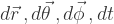 ) Coordinates
![\vec{ds^2}\; = \; [\vec{d{r^2}}\;\;+\;\;\vec{ds^2_{Map}}_{\theta \, \phi}]\;\;=\;\; [\vec{d{r^2}}\;\;+\;\;\vec{d{r^2}}_{\theta}\;\;+\;\;\vec{d{r^2}}_{\phi}]\; =\;](https://s0.wp.com/latex.php?latex=%5Cvec%7Bds%5E2%7D%5C%3B+%3D+%5C%3B+%5B%5Cvec%7Bd%7Br%5E2%7D%7D%5C%3B%5C%3B%2B%5C%3B%5C%3B%5Cvec%7Bds%5E2_%7BMap%7D%7D_%7B%5Ctheta+%5C%2C+%5Cphi%7D%5D%5C%3B%5C%3B%3D%5C%3B%5C%3B+%5B%5Cvec%7Bd%7Br%5E2%7D%7D%5C%3B%5C%3B%2B%5C%3B%5C%3B%5Cvec%7Bd%7Br%5E2%7D%7D_%7B%5Ctheta%7D%5C%3B%5C%3B%2B%5C%3B%5C%3B%5Cvec%7Bd%7Br%5E2%7D%7D_%7B%5Cphi%7D%5D%5C%3B+%3D%5C%3B&bg=ffffff&fg=333333&s=1&c=20201002)
![\vec{ds^2}\;=\;\vec{c^2_{Light}}\,{dt'^2_{Light(s)}}\;=\; [{dr^2}\;\;+\;\;{r^2}\;d\theta^2_{Lat}\;\;+\;\;{r^2}\,sin^2\theta_{Lat}\,d\phi^2_{Lon}]\;](https://s0.wp.com/latex.php?latex=%5Cvec%7Bds%5E2%7D%5C%3B%3D%5C%3B%5Cvec%7Bc%5E2_%7BLight%7D%7D%5C%2C%7Bdt%27%5E2_%7BLight%28s%29%7D%7D%5C%3B%3D%5C%3B+%5B%7Bdr%5E2%7D%5C%3B%5C%3B%2B%5C%3B%5C%3B%7Br%5E2%7D%5C%3Bd%5Ctheta%5E2_%7BLat%7D%5C%3B%5C%3B%2B%5C%3B%5C%3B%7Br%5E2%7D%5C%2Csin%5E2%5Ctheta_%7BLat%7D%5C%2Cd%5Cphi%5E2_%7BLon%7D%5D%5C%3B&bg=ffffff&fg=333333&s=1&c=20201002)
![\vec{ds^2}\;=\; [{dx^2}\;\;+\;\;{dy^2}\;\;+\;\;{dz^2}\;\;+\;\;{r^2}\;d\theta^2_{Lat}\;\;+\;\;{r^2}\,sin^2\theta_{Lat}\,d\phi^2_{Lon}]\;](https://s0.wp.com/latex.php?latex=%5Cvec%7Bds%5E2%7D%5C%3B%3D%5C%3B+%5B%7Bdx%5E2%7D%5C%3B%5C%3B%2B%5C%3B%5C%3B%7Bdy%5E2%7D%5C%3B%5C%3B%2B%5C%3B%5C%3B%7Bdz%5E2%7D%5C%3B%5C%3B%2B%5C%3B%5C%3B%7Br%5E2%7D%5C%3Bd%5Ctheta%5E2_%7BLat%7D%5C%3B%5C%3B%2B%5C%3B%5C%3B%7Br%5E2%7D%5C%2Csin%5E2%5Ctheta_%7BLat%7D%5C%2Cd%5Cphi%5E2_%7BLon%7D%5D%5C%3B&bg=ffffff&fg=333333&s=1&c=20201002)
![\vec{ds^2}\;=\;\vec{c^2_{Light}}\,{dt'^2_{Light(s)}}\;=\;[{dx'^2_{s}}\;+\;{dy'^2_{s}}\;+\;{dz'^2_{s}}] \;](https://s0.wp.com/latex.php?latex=%5Cvec%7Bds%5E2%7D%5C%3B%3D%5C%3B%5Cvec%7Bc%5E2_%7BLight%7D%7D%5C%2C%7Bdt%27%5E2_%7BLight%28s%29%7D%7D%5C%3B%3D%5C%3B%5B%7Bdx%27%5E2_%7Bs%7D%7D%5C%3B%2B%5C%3B%7Bdy%27%5E2_%7Bs%7D%7D%5C%3B%2B%5C%3B%7Bdz%27%5E2_%7Bs%7D%7D%5D+%5C%3B&bg=ffffff&fg=333333&s=1&c=20201002)
 ), and one (1) “geodesic arc-length” component, which is the “Map/Patch/Manifold geodesic metric” (
 ), and the “Longitude Angle Metric” (
 )
)![\vec{ds^2}\; = \; [\vec{d{r^2}}\;\;+\;\;\vec{ds^2_{Map}}_{\theta \, \phi}]\;\;=\;\; [\vec{d{r^2}}\;\;+\;\;{r}\,{\vec{d\Omega_{Map}}_{(\theta \phi)}}]\; =\;](https://s0.wp.com/latex.php?latex=%5Cvec%7Bds%5E2%7D%5C%3B+%3D+%5C%3B+%5B%5Cvec%7Bd%7Br%5E2%7D%7D%5C%3B%5C%3B%2B%5C%3B%5C%3B%5Cvec%7Bds%5E2_%7BMap%7D%7D_%7B%5Ctheta+%5C%2C+%5Cphi%7D%5D%5C%3B%5C%3B%3D%5C%3B%5C%3B+%5B%5Cvec%7Bd%7Br%5E2%7D%7D%5C%3B%5C%3B%2B%5C%3B%5C%3B%7Br%7D%5C%2C%7B%5Cvec%7Bd%5COmega_%7BMap%7D%7D_%7B%28%5Ctheta+%5Cphi%29%7D%7D%5D%5C%3B+%3D%5C%3B&bg=ffffff&fg=333333&s=1&c=20201002)
![\vec{ds^2}\; = \; [\vec{d{r^2}}\;\;+\;\;\vec{ds^2_{Map}}_{\theta \, \phi}]\;\;=\;\; [\vec{d{r^2}}\;\;-\;\; [{(\frac{2(\frac{|v|_{CM}}{c_{Light}})}{1 \;\;+\;\;\frac{|v|_{CM}}{c_{Light}}})}]\vec{dr^2}\; =\;](https://s0.wp.com/latex.php?latex=%5Cvec%7Bds%5E2%7D%5C%3B+%3D+%5C%3B+%5B%5Cvec%7Bd%7Br%5E2%7D%7D%5C%3B%5C%3B%2B%5C%3B%5C%3B%5Cvec%7Bds%5E2_%7BMap%7D%7D_%7B%5Ctheta+%5C%2C+%5Cphi%7D%5D%5C%3B%5C%3B%3D%5C%3B%5C%3B+%5B%5Cvec%7Bd%7Br%5E2%7D%7D%5C%3B%5C%3B-%5C%3B%5C%3B+%5B%7B%28%5Cfrac%7B2%28%5Cfrac%7B%7Cv%7C_%7BCM%7D%7D%7Bc_%7BLight%7D%7D%29%7D%7B1+%5C%3B%5C%3B%2B%5C%3B%5C%3B%5Cfrac%7B%7Cv%7C_%7BCM%7D%7D%7Bc_%7BLight%7D%7D%7D%29%7D%5D%5Cvec%7Bdr%5E2%7D%5C%3B+%3D%5C%3B&bg=ffffff&fg=333333&s=1&c=20201002)


![\vec{ds^2}\;=\;\frac{(-)[\vec{dr^2}\;\;+\;\;[\frac{(1 \;\;+\;\;\frac{|v|_{CM}}{c_{Light}})}{2(\frac{c_{Light}}{|v|_{CM}})}]\,\vec{ds^2_{Map}}_{\theta \, \phi}]}{(1 \;\;-\;\;\frac{|v|^2_{CM}}{c^2_{Light}})}\;=\;\frac{(-)[\vec{dr^2}\;\;-\;\;[\frac{(1 \;\;+\;\;\frac{|v|_{CM}}{c_{Light}})}{2(\frac{c_{Light}}{|v|_{CM}})}]\,\vec{c^2_{Light}}\,{dt^2_{Map}}]}{(1 \;\;-\;\;\frac{|v|^2_{CM}}{c^2_{Light}})}](https://s0.wp.com/latex.php?latex=%5Cvec%7Bds%5E2%7D%5C%3B%3D%5C%3B%5Cfrac%7B%28-%29%5B%5Cvec%7Bdr%5E2%7D%5C%3B%5C%3B%2B%5C%3B%5C%3B%5B%5Cfrac%7B%281+%5C%3B%5C%3B%2B%5C%3B%5C%3B%5Cfrac%7B%7Cv%7C_%7BCM%7D%7D%7Bc_%7BLight%7D%7D%29%7D%7B2%28%5Cfrac%7Bc_%7BLight%7D%7D%7B%7Cv%7C_%7BCM%7D%7D%29%7D%5D%5C%2C%5Cvec%7Bds%5E2_%7BMap%7D%7D_%7B%5Ctheta+%5C%2C+%5Cphi%7D%5D%7D%7B%281+%5C%3B%5C%3B-%5C%3B%5C%3B%5Cfrac%7B%7Cv%7C%5E2_%7BCM%7D%7D%7Bc%5E2_%7BLight%7D%7D%29%7D%5C%3B%3D%5C%3B%5Cfrac%7B%28-%29%5B%5Cvec%7Bdr%5E2%7D%5C%3B%5C%3B-%5C%3B%5C%3B%5B%5Cfrac%7B%281+%5C%3B%5C%3B%2B%5C%3B%5C%3B%5Cfrac%7B%7Cv%7C_%7BCM%7D%7D%7Bc_%7BLight%7D%7D%29%7D%7B2%28%5Cfrac%7Bc_%7BLight%7D%7D%7B%7Cv%7C_%7BCM%7D%7D%29%7D%5D%5C%2C%5Cvec%7Bc%5E2_%7BLight%7D%7D%5C%2C%7Bdt%5E2_%7BMap%7D%7D%5D%7D%7B%281+%5C%3B%5C%3B-%5C%3B%5C%3B%5Cfrac%7B%7Cv%7C%5E2_%7BCM%7D%7D%7Bc%5E2_%7BLight%7D%7D%29%7D&bg=ffffff&fg=333333&s=1&c=20201002)

![{dt'^2_{Light(s)}}\;=\;[{dt^2_{Light}}\;\;-\;\;{dt^2_{Map}}]\;=\;[{dt^2_{Light}}\;\;+\;\;\frac{(\vec{ds_{Map}}_{\theta \, \phi})^2}{c^2_{Light}}]](https://s0.wp.com/latex.php?latex=%7Bdt%27%5E2_%7BLight%28s%29%7D%7D%5C%3B%3D%5C%3B%5B%7Bdt%5E2_%7BLight%7D%7D%5C%3B%5C%3B-%5C%3B%5C%3B%7Bdt%5E2_%7BMap%7D%7D%5D%5C%3B%3D%5C%3B%5B%7Bdt%5E2_%7BLight%7D%7D%5C%3B%5C%3B%2B%5C%3B%5C%3B%5Cfrac%7B%28%5Cvec%7Bds_%7BMap%7D%7D_%7B%5Ctheta+%5C%2C+%5Cphi%7D%29%5E2%7D%7Bc%5E2_%7BLight%7D%7D%5D&bg=ffffff&fg=333333&s=1&c=20201002)
 ) – measured in the “External Observer” frame of reference, and described as function of the
 ![{dt'^2_{Light(s)}}\;=\;{dt^2_{Light}}[\frac{1 \;\;-\;\;\frac{|v|_{CM}}{c_{Light}}}{1 \;\;+\;\;\frac{|v|_{CM}}{c_{Light}}}]\;\;=\;\;{dt^2_{Map}}[\frac{1 \;\;-\;\;\frac{|v|_{CM}}{c_{Light}}}{2(\frac{|v|_{CM}}{c_{Light}})}]\;](https://s0.wp.com/latex.php?latex=%7Bdt%27%5E2_%7BLight%28s%29%7D%7D%5C%3B%3D%5C%3B%7Bdt%5E2_%7BLight%7D%7D%5B%5Cfrac%7B1+%5C%3B%5C%3B-%5C%3B%5C%3B%5Cfrac%7B%7Cv%7C_%7BCM%7D%7D%7Bc_%7BLight%7D%7D%7D%7B1+%5C%3B%5C%3B%2B%5C%3B%5C%3B%5Cfrac%7B%7Cv%7C_%7BCM%7D%7D%7Bc_%7BLight%7D%7D%7D%5D%5C%3B%5C%3B%3D%5C%3B%5C%3B%7Bdt%5E2_%7BMap%7D%7D%5B%5Cfrac%7B1+%5C%3B%5C%3B-%5C%3B%5C%3B%5Cfrac%7B%7Cv%7C_%7BCM%7D%7D%7Bc_%7BLight%7D%7D%7D%7B2%28%5Cfrac%7B%7Cv%7C_%7BCM%7D%7D%7Bc_%7BLight%7D%7D%29%7D%5D%5C%3B&bg=ffffff&fg=333333&s=1&c=20201002)
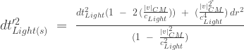
![{dt'^2_{Light(s)}}\;=\;\frac{(-)[{dt^2_{Light}}\;\;+\;\;(\frac{1}{c^2_{Light}})[\frac{(1 \;\;+\;\;\frac{|v|_{CM}}{c_{Light}})}{2(\frac{c_{Light}}{|v|_{CM}})}]\,\vec{ds^2_{Map}}_{\theta \, \phi}]}{(1 \;\;-\;\;\frac{|v|^2_{CM}}{c^2_{Light}})}\;=\;\frac{(-)[{dt^2_{Light}}\;\;-\;\;[\frac{(1 \;\;+\;\;\frac{|v|_{CM}}{c_{Light}})}{2(\frac{c_{Light}}{|v|_{CM}})}]\,{dt^2_{Map}}]}{(1 \;\;-\;\;\frac{|v|^2_{CM}}{c^2_{Light}})}](https://s0.wp.com/latex.php?latex=%7Bdt%27%5E2_%7BLight%28s%29%7D%7D%5C%3B%3D%5C%3B%5Cfrac%7B%28-%29%5B%7Bdt%5E2_%7BLight%7D%7D%5C%3B%5C%3B%2B%5C%3B%5C%3B%28%5Cfrac%7B1%7D%7Bc%5E2_%7BLight%7D%7D%29%5B%5Cfrac%7B%281+%5C%3B%5C%3B%2B%5C%3B%5C%3B%5Cfrac%7B%7Cv%7C_%7BCM%7D%7D%7Bc_%7BLight%7D%7D%29%7D%7B2%28%5Cfrac%7Bc_%7BLight%7D%7D%7B%7Cv%7C_%7BCM%7D%7D%29%7D%5D%5C%2C%5Cvec%7Bds%5E2_%7BMap%7D%7D_%7B%5Ctheta+%5C%2C+%5Cphi%7D%5D%7D%7B%281+%5C%3B%5C%3B-%5C%3B%5C%3B%5Cfrac%7B%7Cv%7C%5E2_%7BCM%7D%7D%7Bc%5E2_%7BLight%7D%7D%29%7D%5C%3B%3D%5C%3B%5Cfrac%7B%28-%29%5B%7Bdt%5E2_%7BLight%7D%7D%5C%3B%5C%3B-%5C%3B%5C%3B%5B%5Cfrac%7B%281+%5C%3B%5C%3B%2B%5C%3B%5C%3B%5Cfrac%7B%7Cv%7C_%7BCM%7D%7D%7Bc_%7BLight%7D%7D%29%7D%7B2%28%5Cfrac%7Bc_%7BLight%7D%7D%7B%7Cv%7C_%7BCM%7D%7D%29%7D%5D%5C%2C%7Bdt%5E2_%7BMap%7D%7D%5D%7D%7B%281+%5C%3B%5C%3B-%5C%3B%5C%3B%5Cfrac%7B%7Cv%7C%5E2_%7BCM%7D%7D%7Bc%5E2_%7BLight%7D%7D%29%7D&bg=ffffff&fg=333333&s=1&c=20201002)

 ) Coordinates
![\vec{d\Omega^2_{Map}}_{(\theta \phi)}\; =\; [\frac{\vec{d{r^2}}_{\theta}}{r^2}\;\;+\;\;\frac{\vec{d{r^2}}_{\phi}}{r^2}]\;=\;[\vec{d\theta^2_{Lat}}\;\;+\;\; \sin^2\theta_{Lat}\,\vec{d\phi^2_{Lon}}]\;](https://s0.wp.com/latex.php?latex=%5Cvec%7Bd%5COmega%5E2_%7BMap%7D%7D_%7B%28%5Ctheta+%5Cphi%29%7D%5C%3B+%3D%5C%3B+%5B%5Cfrac%7B%5Cvec%7Bd%7Br%5E2%7D%7D_%7B%5Ctheta%7D%7D%7Br%5E2%7D%5C%3B%5C%3B%2B%5C%3B%5C%3B%5Cfrac%7B%5Cvec%7Bd%7Br%5E2%7D%7D_%7B%5Cphi%7D%7D%7Br%5E2%7D%5D%5C%3B%3D%5C%3B%5B%5Cvec%7Bd%5Ctheta%5E2_%7BLat%7D%7D%5C%3B%5C%3B%2B%5C%3B%5C%3B+%5Csin%5E2%5Ctheta_%7BLat%7D%5C%2C%5Cvec%7Bd%5Cphi%5E2_%7BLon%7D%7D%5D%5C%3B&bg=ffffff&fg=333333&s=1&c=20201002)

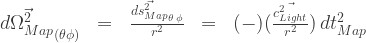
 ) in the
  ) in the
 ![\vec{d\Omega^2_{Map}}_{(\theta \phi)}\;\;=\;\;{\omega^2_{\Omega}}\,{dt^2_{Light}}\;\;=\;{dt^2_{Light}}\,[{\omega^2_{\theta}\;+\;(sin^2\theta_{Lat})\,\omega^2_{\phi}}]](https://s0.wp.com/latex.php?latex=%5Cvec%7Bd%5COmega%5E2_%7BMap%7D%7D_%7B%28%5Ctheta+%5Cphi%29%7D%5C%3B%5C%3B%3D%5C%3B%5C%3B%7B%5Comega%5E2_%7B%5COmega%7D%7D%5C%2C%7Bdt%5E2_%7BLight%7D%7D%5C%3B%5C%3B%3D%5C%3B%7Bdt%5E2_%7BLight%7D%7D%5C%2C%5B%7B%5Comega%5E2_%7B%5Ctheta%7D%5C%3B%2B%5C%3B%28sin%5E2%5Ctheta_%7BLat%7D%29%5C%2C%5Comega%5E2_%7B%5Cphi%7D%7D%5D&bg=ffffff&fg=333333&s=1&c=20201002)
![\vec{d\Omega^2_{Map}}_{(\theta \phi)}\;\;=\;\;{\omega'^2_{\Omega(s)}}\,{dt'^2_{Light(s)}}\;\;=\;\;{dt'^2_{Light(s)}}\,[{\omega'^2_{\theta(s)}\;+\;(sin^2\theta_{Lat})\,\omega'^2_{\phi(s)}}]](https://s0.wp.com/latex.php?latex=%5Cvec%7Bd%5COmega%5E2_%7BMap%7D%7D_%7B%28%5Ctheta+%5Cphi%29%7D%5C%3B%5C%3B%3D%5C%3B%5C%3B%7B%5Comega%27%5E2_%7B%5COmega%28s%29%7D%7D%5C%2C%7Bdt%27%5E2_%7BLight%28s%29%7D%7D%5C%3B%5C%3B%3D%5C%3B%5C%3B%7Bdt%27%5E2_%7BLight%28s%29%7D%7D%5C%2C%5B%7B%5Comega%27%5E2_%7B%5Ctheta%28s%29%7D%5C%3B%2B%5C%3B%28sin%5E2%5Ctheta_%7BLat%7D%29%5C%2C%5Comega%27%5E2_%7B%5Cphi%28s%29%7D%7D%5D&bg=ffffff&fg=333333&s=1&c=20201002)


 ) – is a scalar (direction independent) and is described along the “Latitude” Spherical (
 ) Coordinate. And, likewise is described by the spin, rotation, or torsion on the surface of a sphere, given by the square of the
  ) in the
  ) in the


 ) – is a scalar (direction independent) and is described along the “Longitude” Spherical (
 ) Coordinate. And, likewise is described by the spin, rotation, or torsion on the surface of a sphere, given by the square of the
  ) in the
  ) in the

 ) Cartesian Coordinates
![\vec{ds^2_{Map}}_{\theta \, \phi}\;=\;(-)\vec{c^2_{Light}}\,{dt^2_{Map}}\;=\; [\vec{dx^2_{Map}}\;+\;\vec{dy^2_{Map}}\;+\;\vec{dz^2_{Map}}]](https://s0.wp.com/latex.php?latex=%5Cvec%7Bds%5E2_%7BMap%7D%7D_%7B%5Ctheta+%5C%2C+%5Cphi%7D%5C%3B%3D%5C%3B%28-%29%5Cvec%7Bc%5E2_%7BLight%7D%7D%5C%2C%7Bdt%5E2_%7BMap%7D%7D%5C%3B%3D%5C%3B+%5B%5Cvec%7Bdx%5E2_%7BMap%7D%7D%5C%3B%2B%5C%3B%5Cvec%7Bdy%5E2_%7BMap%7D%7D%5C%3B%2B%5C%3B%5Cvec%7Bdz%5E2_%7BMap%7D%7D%5D&bg=ffffff&fg=333333&s=1&c=20201002)
![\vec{ds^2_{Map}}_{\theta \, \phi}\;=\; [\vec{ds^2}\;-\;\vec{dr^2}]\;=\; [\vec{dx^2_{Map}}\;+\;\vec{dy^2_{Map}}\;+\;\vec{dz^2_{Map}}]](https://s0.wp.com/latex.php?latex=%5Cvec%7Bds%5E2_%7BMap%7D%7D_%7B%5Ctheta+%5C%2C+%5Cphi%7D%5C%3B%3D%5C%3B+%5B%5Cvec%7Bds%5E2%7D%5C%3B-%5C%3B%5Cvec%7Bdr%5E2%7D%5D%5C%3B%3D%5C%3B+%5B%5Cvec%7Bdx%5E2_%7BMap%7D%7D%5C%3B%2B%5C%3B%5Cvec%7Bdy%5E2_%7BMap%7D%7D%5C%3B%2B%5C%3B%5Cvec%7Bdz%5E2_%7BMap%7D%7D%5D&bg=ffffff&fg=333333&s=1&c=20201002)
![\vec{ds^2_{Map}}_{\theta \, \phi}\;=\;(-)\vec{c^2_{Light}}\,{dt^2_{Map}}\;=\; [\vec{c^2_{Light}}\,{dt'^2_{Light(s)}}\;-\;\vec{c^2_{Light}}\,{dt^2_{Light}}]](https://s0.wp.com/latex.php?latex=%5Cvec%7Bds%5E2_%7BMap%7D%7D_%7B%5Ctheta+%5C%2C+%5Cphi%7D%5C%3B%3D%5C%3B%28-%29%5Cvec%7Bc%5E2_%7BLight%7D%7D%5C%2C%7Bdt%5E2_%7BMap%7D%7D%5C%3B%3D%5C%3B+%5B%5Cvec%7Bc%5E2_%7BLight%7D%7D%5C%2C%7Bdt%27%5E2_%7BLight%28s%29%7D%7D%5C%3B-%5C%3B%5Cvec%7Bc%5E2_%7BLight%7D%7D%5C%2C%7Bdt%5E2_%7BLight%7D%7D%5D&bg=ffffff&fg=333333&s=1&c=20201002)
 ) Coordinates
![\vec{ds_{Map}}_{\theta \, \phi}\;=\; [\vec{ds^2}\;-\;\vec{dr^2}]\;=\;\; [\vec{d{r^2}}_{\theta}\;\;+\;\;\vec{d{r^2}}_{\phi}]\; =\;](https://s0.wp.com/latex.php?latex=%5Cvec%7Bds_%7BMap%7D%7D_%7B%5Ctheta+%5C%2C+%5Cphi%7D%5C%3B%3D%5C%3B+%5B%5Cvec%7Bds%5E2%7D%5C%3B-%5C%3B%5Cvec%7Bdr%5E2%7D%5D%5C%3B%3D%5C%3B%5C%3B+%5B%5Cvec%7Bd%7Br%5E2%7D%7D_%7B%5Ctheta%7D%5C%3B%5C%3B%2B%5C%3B%5C%3B%5Cvec%7Bd%7Br%5E2%7D%7D_%7B%5Cphi%7D%5D%5C%3B+%3D%5C%3B&bg=ffffff&fg=333333&s=1&c=20201002)
![\vec{ds^2_{Map}}_{\theta \, \phi}\;=\;(-)\vec{c^2_{Light}}\,{dt^2_{Map}}\;=\; [{r^2}\;d\theta^2_{Lat}\;\;+\;\;{r^2}\,sin^2\theta_{Lat}\,d\phi^2_{Lon}]\;](https://s0.wp.com/latex.php?latex=%5Cvec%7Bds%5E2_%7BMap%7D%7D_%7B%5Ctheta+%5C%2C+%5Cphi%7D%5C%3B%3D%5C%3B%28-%29%5Cvec%7Bc%5E2_%7BLight%7D%7D%5C%2C%7Bdt%5E2_%7BMap%7D%7D%5C%3B%3D%5C%3B+%5B%7Br%5E2%7D%5C%3Bd%5Ctheta%5E2_%7BLat%7D%5C%3B%5C%3B%2B%5C%3B%5C%3B%7Br%5E2%7D%5C%2Csin%5E2%5Ctheta_%7BLat%7D%5C%2Cd%5Cphi%5E2_%7BLon%7D%5D%5C%3B&bg=ffffff&fg=333333&s=1&c=20201002)


\;=\;(-)[{\frac{2(\frac{|v|_{CM}}{c_{Light}})}{1\;\;-\;\;\frac{|v|_{CM}}{c_{Light}}}}]({ds^2})](https://s0.wp.com/latex.php?latex=%5Cvec%7Bds%5E2_%7BMap%7D%7D_%7B%5Ctheta+%5C%2C+%5Cphi%7D%5C%3B%3D%5C%3B%28-%29%5B%7B%5Cfrac%7B2%28%5Cfrac%7B%7Cv%7C_%7BCM%7D%7D%7Bc_%7BLight%7D%7D%29%7D%7B1+%5C%3B%5C%3B%2B%5C%3B%5C%3B%5Cfrac%7B%7Cv%7C_%7BCM%7D%7D%7Bc_%7BLight%7D%7D%7D%7D%5D%28%7Bdr%5E2%7D%29%5C%3B%3D%5C%3B%28-%29%5B%7B%5Cfrac%7B2%28%5Cfrac%7B%7Cv%7C_%7BCM%7D%7D%7Bc_%7BLight%7D%7D%29%7D%7B1%5C%3B%5C%3B-%5C%3B%5C%3B%5Cfrac%7B%7Cv%7C_%7BCM%7D%7D%7Bc_%7BLight%7D%7D%7D%7D%5D%28%7Bds%5E2%7D%29&bg=ffffff&fg=333333&s=1&c=20201002)

 ) – measured in the
 ![{dt^2_{Map}}\;=\;(-)[\frac{\vec{ds^2_{Map}}_{\theta \, \phi}}{\vec{c^2_{Light}}}]\;=\;(-)[\frac{(\vec{ds})^2 \;\;-\;\; (\vec{dr})^2}{\vec{c^2_{Light}}}]\;](https://s0.wp.com/latex.php?latex=%7Bdt%5E2_%7BMap%7D%7D%5C%3B%3D%5C%3B%28-%29%5B%5Cfrac%7B%5Cvec%7Bds%5E2_%7BMap%7D%7D_%7B%5Ctheta+%5C%2C+%5Cphi%7D%7D%7B%5Cvec%7Bc%5E2_%7BLight%7D%7D%7D%5D%5C%3B%3D%5C%3B%28-%29%5B%5Cfrac%7B%28%5Cvec%7Bds%7D%29%5E2+%5C%3B%5C%3B-%5C%3B%5C%3B+%28%5Cvec%7Bdr%7D%29%5E2%7D%7B%5Cvec%7Bc%5E2_%7BLight%7D%7D%7D%5D%5C%3B&bg=ffffff&fg=333333&s=1&c=20201002)
![{dt^2_{Map}}\;=\;(-)[{({dt'_{Light(s)}})^2\;-\;({dt_{Light}})^2}]\;](https://s0.wp.com/latex.php?latex=%7Bdt%5E2_%7BMap%7D%7D%5C%3B%3D%5C%3B%28-%29%5B%7B%28%7Bdt%27_%7BLight%28s%29%7D%7D%29%5E2%5C%3B-%5C%3B%28%7Bdt_%7BLight%7D%7D%29%5E2%7D%5D%5C%3B&bg=ffffff&fg=333333&s=1&c=20201002)
![{dt^2_{Map}}\;=\;(-)[\frac{{r^2}\,{\vec{d\Omega^2_{Map}}_{(\theta \phi)}}}{\vec{c^2_{Light}}}]\;](https://s0.wp.com/latex.php?latex=%7Bdt%5E2_%7BMap%7D%7D%5C%3B%3D%5C%3B%28-%29%5B%5Cfrac%7B%7Br%5E2%7D%5C%2C%7B%5Cvec%7Bd%5COmega%5E2_%7BMap%7D%7D_%7B%28%5Ctheta+%5Cphi%29%7D%7D%7D%7B%5Cvec%7Bc%5E2_%7BLight%7D%7D%7D%5D%5C%3B&bg=ffffff&fg=333333&s=1&c=20201002)
![{dt^2_{Map}}\;=\;\;{dt^2_{Light}}[{\frac{2(\frac{|v|_{CM}}{c_{Light}})}{1 \;\;+\;\;\frac{|v|_{CM}}{c_{Light}}}}]\;\;=\;\;{dt'^2_{Light(s)}}[{\frac{2(\frac{|v|_{CM}}{c_{Light}})}{1 \;\;-\;\;\frac{|v|_{CM}}{c_{Light}}}}]\;](https://s0.wp.com/latex.php?latex=%7Bdt%5E2_%7BMap%7D%7D%5C%3B%3D%5C%3B%5C%3B%7Bdt%5E2_%7BLight%7D%7D%5B%7B%5Cfrac%7B2%28%5Cfrac%7B%7Cv%7C_%7BCM%7D%7D%7Bc_%7BLight%7D%7D%29%7D%7B1+%5C%3B%5C%3B%2B%5C%3B%5C%3B%5Cfrac%7B%7Cv%7C_%7BCM%7D%7D%7Bc_%7BLight%7D%7D%7D%7D%5D%5C%3B%5C%3B%3D%5C%3B%5C%3B%7Bdt%27%5E2_%7BLight%28s%29%7D%7D%5B%7B%5Cfrac%7B2%28%5Cfrac%7B%7Cv%7C_%7BCM%7D%7D%7Bc_%7BLight%7D%7D%29%7D%7B1+%5C%3B%5C%3B-%5C%3B%5C%3B%5Cfrac%7B%7Cv%7C_%7BCM%7D%7D%7Bc_%7BLight%7D%7D%7D%7D%5D%5C%3B&bg=ffffff&fg=333333&s=1&c=20201002)
![{dt^2_{Map}}\;=\;\;{dr^2}[{\frac{2(\frac{|v|_{CM}}{c^3_{Light}})}{1 \;\;+\;\;\frac{|v|_{CM}}{c_{Light}}}}]\;\;=\;\;{ds^2}[{\frac{2(\frac{|v|_{CM}}{c^3_{Light}})}{1 \;\;-\;\;\frac{|v|_{CM}}{c_{Light}}}}]\;](https://s0.wp.com/latex.php?latex=%7Bdt%5E2_%7BMap%7D%7D%5C%3B%3D%5C%3B%5C%3B%7Bdr%5E2%7D%5B%7B%5Cfrac%7B2%28%5Cfrac%7B%7Cv%7C_%7BCM%7D%7D%7Bc%5E3_%7BLight%7D%7D%29%7D%7B1+%5C%3B%5C%3B%2B%5C%3B%5C%3B%5Cfrac%7B%7Cv%7C_%7BCM%7D%7D%7Bc_%7BLight%7D%7D%7D%7D%5D%5C%3B%5C%3B%3D%5C%3B%5C%3B%7Bds%5E2%7D%5B%7B%5Cfrac%7B2%28%5Cfrac%7B%7Cv%7C_%7BCM%7D%7D%7Bc%5E3_%7BLight%7D%7D%29%7D%7B1+%5C%3B%5C%3B-%5C%3B%5C%3B%5Cfrac%7B%7Cv%7C_%7BCM%7D%7D%7Bc_%7BLight%7D%7D%7D%7D%5D%5C%3B&bg=ffffff&fg=333333&s=1&c=20201002)
 ), and relative to the
 ![{dt^2_{Map}}\;=\;\;{d\tau^2_{Sync}}[{\frac{2(\frac{c_{Light}}{|v|_{CM}})}{1 \;\;+\;\;\frac{|v|_{CM}}{c_{Light}}}}]\;\;=\;\;{d\tau'^2_{Sync}}[{\frac{2(\frac{c_{Light}}{|v|_{CM}})}{1 \;\;-\;\;\frac{|v|_{CM}}{c_{Light}}}}]\;](https://s0.wp.com/latex.php?latex=%7Bdt%5E2_%7BMap%7D%7D%5C%3B%3D%5C%3B%5C%3B%7Bd%5Ctau%5E2_%7BSync%7D%7D%5B%7B%5Cfrac%7B2%28%5Cfrac%7Bc_%7BLight%7D%7D%7B%7Cv%7C_%7BCM%7D%7D%29%7D%7B1+%5C%3B%5C%3B%2B%5C%3B%5C%3B%5Cfrac%7B%7Cv%7C_%7BCM%7D%7D%7Bc_%7BLight%7D%7D%7D%7D%5D%5C%3B%5C%3B%3D%5C%3B%5C%3B%7Bd%5Ctau%27%5E2_%7BSync%7D%7D%5B%7B%5Cfrac%7B2%28%5Cfrac%7Bc_%7BLight%7D%7D%7B%7Cv%7C_%7BCM%7D%7D%29%7D%7B1+%5C%3B%5C%3B-%5C%3B%5C%3B%5Cfrac%7B%7Cv%7C_%7BCM%7D%7D%7Bc_%7BLight%7D%7D%7D%7D%5D%5C%3B&bg=ffffff&fg=333333&s=1&c=20201002)
![{dt^2_{Map}}\;=\;\;((\frac{{|v|^2_{CM}}}{{c^4_{Light}} }){dr^2})[{\frac{2(\frac{c_{Light}}{|v|_{CM}})}{1 \;\;+\;\;\frac{|v|_{CM}}{c_{Light}}}}]\;\;=\;\;((\frac{{|v|^2_{CM}}}{{c^4_{Light}} }){ds^2})[{\frac{2(\frac{c_{Light}}{|v|_{CM}})}{1 \;\;-\;\;\frac{|v|_{CM}}{c_{Light}}}}]\;](https://s0.wp.com/latex.php?latex=%7Bdt%5E2_%7BMap%7D%7D%5C%3B%3D%5C%3B%5C%3B%28%28%5Cfrac%7B%7B%7Cv%7C%5E2_%7BCM%7D%7D%7D%7B%7Bc%5E4_%7BLight%7D%7D+%7D%29%7Bdr%5E2%7D%29%5B%7B%5Cfrac%7B2%28%5Cfrac%7Bc_%7BLight%7D%7D%7B%7Cv%7C_%7BCM%7D%7D%29%7D%7B1+%5C%3B%5C%3B%2B%5C%3B%5C%3B%5Cfrac%7B%7Cv%7C_%7BCM%7D%7D%7Bc_%7BLight%7D%7D%7D%7D%5D%5C%3B%5C%3B%3D%5C%3B%5C%3B%28%28%5Cfrac%7B%7B%7Cv%7C%5E2_%7BCM%7D%7D%7D%7B%7Bc%5E4_%7BLight%7D%7D+%7D%29%7Bds%5E2%7D%29%5B%7B%5Cfrac%7B2%28%5Cfrac%7Bc_%7BLight%7D%7D%7B%7Cv%7C_%7BCM%7D%7D%29%7D%7B1+%5C%3B%5C%3B-%5C%3B%5C%3B%5Cfrac%7B%7Cv%7C_%7BCM%7D%7D%7Bc_%7BLight%7D%7D%7D%7D%5D%5C%3B&bg=ffffff&fg=333333&s=1&c=20201002)
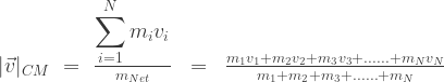
![{|\vec{v}|_{CM}} \,\, =\,\,(-){c_{Light}}[\frac{(\vec{d\Omega_{Map}}_{(\theta \phi)})^2}{2\,(\frac{\vec{dr}}{r})^2\;\;+\;\;(\vec{d\Omega_{Map}}_{(\theta \phi)})^2}]](https://s0.wp.com/latex.php?latex=%7B%7C%5Cvec%7Bv%7D%7C_%7BCM%7D%7D+%5C%2C%5C%2C+%3D%5C%2C%5C%2C%28-%29%7Bc_%7BLight%7D%7D%5B%5Cfrac%7B%28%5Cvec%7Bd%5COmega_%7BMap%7D%7D_%7B%28%5Ctheta+%5Cphi%29%7D%29%5E2%7D%7B2%5C%2C%28%5Cfrac%7B%5Cvec%7Bdr%7D%7D%7Br%7D%29%5E2%5C%3B%5C%3B%2B%5C%3B%5C%3B%28%5Cvec%7Bd%5COmega_%7BMap%7D%7D_%7B%28%5Ctheta+%5Cphi%29%7D%29%5E2%7D%5D&bg=ffffff&fg=333333&s=1&c=20201002)
![{|\vec{v}|_{CM}}\,\,=\,\,(-){c_{Light}}[\frac{(\vec{d\Omega_{Map}}_{(\theta \phi)})^2}{2\,(\frac{\vec{ds}}{s})^2\;\;+\;\;(\vec{d\Omega_{Map}}_{(\theta \phi)})^2}]](https://s0.wp.com/latex.php?latex=%7B%7C%5Cvec%7Bv%7D%7C_%7BCM%7D%7D%5C%2C%5C%2C%3D%5C%2C%5C%2C%28-%29%7Bc_%7BLight%7D%7D%5B%5Cfrac%7B%28%5Cvec%7Bd%5COmega_%7BMap%7D%7D_%7B%28%5Ctheta+%5Cphi%29%7D%29%5E2%7D%7B2%5C%2C%28%5Cfrac%7B%5Cvec%7Bds%7D%7D%7Bs%7D%29%5E2%5C%3B%5C%3B%2B%5C%3B%5C%3B%28%5Cvec%7Bd%5COmega_%7BMap%7D%7D_%7B%28%5Ctheta+%5Cphi%29%7D%29%5E2%7D%5D&bg=ffffff&fg=333333&s=0&c=20201002)
![{|\vec{v}|_{CM}}\;\;=\;\;(-){c_{Light}}[\frac{(\vec{\int{d\Omega_{Map}}_{(\theta \phi)}})^2}{2\,(\int_C^s{\frac{\vec{ds}}{s}})^2\;\;+\;\;(\int{\vec{d\Omega_{Map}}_{(\theta \phi)}})^2}]](https://s0.wp.com/latex.php?latex=%7B%7C%5Cvec%7Bv%7D%7C_%7BCM%7D%7D%5C%3B%5C%3B%3D%5C%3B%5C%3B%28-%29%7Bc_%7BLight%7D%7D%5B%5Cfrac%7B%28%5Cvec%7B%5Cint%7Bd%5COmega_%7BMap%7D%7D_%7B%28%5Ctheta+%5Cphi%29%7D%7D%29%5E2%7D%7B2%5C%2C%28%5Cint_C%5Es%7B%5Cfrac%7B%5Cvec%7Bds%7D%7D%7Bs%7D%7D%29%5E2%5C%3B%5C%3B%2B%5C%3B%5C%3B%28%5Cint%7B%5Cvec%7Bd%5COmega_%7BMap%7D%7D_%7B%28%5Ctheta+%5Cphi%29%7D%7D%29%5E2%7D%5D&bg=ffffff&fg=333333&s=0&c=20201002)
![{|\vec{v}|_{CM}} \,\, =\,\,(-){c_{Light}}[\frac{({\Omega_{Map}}_{(\theta \phi)})^2}{2\,(ln(\frac{s}{{r_{Schwarzschild}}}))^2\;\;+\;\;({\Omega_{Map}}_{(\theta \phi)})^2}]](https://s0.wp.com/latex.php?latex=%7B%7C%5Cvec%7Bv%7D%7C_%7BCM%7D%7D+%5C%2C%5C%2C+%3D%5C%2C%5C%2C%28-%29%7Bc_%7BLight%7D%7D%5B%5Cfrac%7B%28%7B%5COmega_%7BMap%7D%7D_%7B%28%5Ctheta+%5Cphi%29%7D%29%5E2%7D%7B2%5C%2C%28ln%28%5Cfrac%7Bs%7D%7B%7Br_%7BSchwarzschild%7D%7D%7D%29%29%5E2%5C%3B%5C%3B%2B%5C%3B%5C%3B%28%7B%5COmega_%7BMap%7D%7D_%7B%28%5Ctheta+%5Cphi%29%7D%29%5E2%7D%5D&bg=ffffff&fg=333333&s=1&c=20201002)
![{r^2}\,\,=\,\,{r^2_{Schwarzschild}}\,{e^{(-)\,{\Omega^2_{Map}}_{(\theta \phi)}[{{\frac{1}{2}}(1\;\;+\;\; \frac{c_{Light}}{|\vec{v}|_{CM}})}]}}](https://s0.wp.com/latex.php?latex=%7Br%5E2%7D%5C%2C%5C%2C%3D%5C%2C%5C%2C%7Br%5E2_%7BSchwarzschild%7D%7D%5C%2C%7Be%5E%7B%28-%29%5C%2C%7B%5COmega%5E2_%7BMap%7D%7D_%7B%28%5Ctheta+%5Cphi%29%7D%5B%7B%7B%5Cfrac%7B1%7D%7B2%7D%7D%281%5C%3B%5C%3B%2B%5C%3B%5C%3B+%5Cfrac%7Bc_%7BLight%7D%7D%7B%7C%5Cvec%7Bv%7D%7C_%7BCM%7D%7D%29%7D%5D%7D%7D&bg=ffffff&fg=333333&s=1&c=20201002)

![{r^2}\;\;=\;\;(\frac{4\,{m^2_{Net}}\,G^2}{c^4_{Light}})\,{e^{(-)\,[{{\theta^2_{Lat}}\;\;+\;\; \sin^2\theta_{Lat}\,{\phi^2_{Lon}]}}[{{\frac{1}{2}}(1\;\;+\;\; \frac{c_{Light}}{|\vec{v}|_{CM}})}]}}](https://s0.wp.com/latex.php?latex=%7Br%5E2%7D%5C%3B%5C%3B%3D%5C%3B%5C%3B%28%5Cfrac%7B4%5C%2C%7Bm%5E2_%7BNet%7D%7D%5C%2CG%5E2%7D%7Bc%5E4_%7BLight%7D%7D%29%5C%2C%7Be%5E%7B%28-%29%5C%2C%5B%7B%7B%5Ctheta%5E2_%7BLat%7D%7D%5C%3B%5C%3B%2B%5C%3B%5C%3B+%5Csin%5E2%5Ctheta_%7BLat%7D%5C%2C%7B%5Cphi%5E2_%7BLon%7D%5D%7D%7D%5B%7B%7B%5Cfrac%7B1%7D%7B2%7D%7D%281%5C%3B%5C%3B%2B%5C%3B%5C%3B+%5Cfrac%7Bc_%7BLight%7D%7D%7B%7C%5Cvec%7Bv%7D%7C_%7BCM%7D%7D%29%7D%5D%7D%7D&bg=ffffff&fg=333333&s=1&c=20201002)
![{s^2}\,\,=\,\,{r^2}\,[{1\;\;+\;\;{\Omega^2_{Map}}_{(\theta \phi)}}]](https://s0.wp.com/latex.php?latex=%7Bs%5E2%7D%5C%2C%5C%2C%3D%5C%2C%5C%2C%7Br%5E2%7D%5C%2C%5B%7B1%5C%3B%5C%3B%2B%5C%3B%5C%3B%7B%5COmega%5E2_%7BMap%7D%7D_%7B%28%5Ctheta+%5Cphi%29%7D%7D%5D&bg=ffffff&fg=333333&s=1&c=20201002)
![{s^2}\,\,=\,\,{r^2_{Schwarzschild}}\,[{1\;+\;{\theta^2_{Lat}}\;+\; \sin^2\theta_{Lat}\,{\phi^2_{Lon}}}]\,{e^{(-)\,[{{\theta^2_{Lat}}\;\;+\;\; \sin^2\theta_{Lat}\,{\phi^2_{Lon}}}][{{\frac{1}{2}}(1\;\;+\;\; \frac{c_{Light}}{|\vec{v}|_{CM}})}]}}](https://s0.wp.com/latex.php?latex=%7Bs%5E2%7D%5C%2C%5C%2C%3D%5C%2C%5C%2C%7Br%5E2_%7BSchwarzschild%7D%7D%5C%2C%5B%7B1%5C%3B%2B%5C%3B%7B%5Ctheta%5E2_%7BLat%7D%7D%5C%3B%2B%5C%3B+%5Csin%5E2%5Ctheta_%7BLat%7D%5C%2C%7B%5Cphi%5E2_%7BLon%7D%7D%7D%5D%5C%2C%7Be%5E%7B%28-%29%5C%2C%5B%7B%7B%5Ctheta%5E2_%7BLat%7D%7D%5C%3B%5C%3B%2B%5C%3B%5C%3B+%5Csin%5E2%5Ctheta_%7BLat%7D%5C%2C%7B%5Cphi%5E2_%7BLon%7D%7D%7D%5D%5B%7B%7B%5Cfrac%7B1%7D%7B2%7D%7D%281%5C%3B%5C%3B%2B%5C%3B%5C%3B+%5Cfrac%7Bc_%7BLight%7D%7D%7B%7C%5Cvec%7Bv%7D%7C_%7BCM%7D%7D%29%7D%5D%7D%7D&bg=ffffff&fg=333333&s=1&c=20201002)
![{s^2_{Map}}_{\theta \, \phi}\,\,=\,\,{r^2}\,{\Omega^2_{Map}}_{(\theta \phi)}\,\,=\,\,{r^2}\, [{{\theta^2_{Lat}}\;\;+\;\;\sin^2\theta_{Lat}\,{\phi^2_{Lon}}}]](https://s0.wp.com/latex.php?latex=%7Bs%5E2_%7BMap%7D%7D_%7B%5Ctheta+%5C%2C+%5Cphi%7D%5C%2C%5C%2C%3D%5C%2C%5C%2C%7Br%5E2%7D%5C%2C%7B%5COmega%5E2_%7BMap%7D%7D_%7B%28%5Ctheta+%5Cphi%29%7D%5C%2C%5C%2C%3D%5C%2C%5C%2C%7Br%5E2%7D%5C%2C+%5B%7B%7B%5Ctheta%5E2_%7BLat%7D%7D%5C%3B%5C%3B%2B%5C%3B%5C%3B%5Csin%5E2%5Ctheta_%7BLat%7D%5C%2C%7B%5Cphi%5E2_%7BLon%7D%7D%7D%5D&bg=ffffff&fg=333333&s=1&c=20201002)
![{s^2_{Map}}_{\theta \, \phi}\,\,=\,\,(-){r^2}\,[\frac{(ln(\frac{r}{{r_{Schwarzschild}}}))^2}{{{\frac{1}{2}}(1\;\;+\;\; \frac{c_{Light}}{|\vec{v}|_{CM}})}}]\,\,=\,\,(-){\frac{m_{Net}\,G}{g_{Gravity}}}\,[\frac{(ln(\frac{r}{{r_{Schwarzschild}}}))^2}{{{\frac{1}{2}}(1\;\;+\;\; \frac{c_{Light}}{|\vec{v}|_{CM}})}}]](https://s0.wp.com/latex.php?latex=%7Bs%5E2_%7BMap%7D%7D_%7B%5Ctheta+%5C%2C+%5Cphi%7D%5C%2C%5C%2C%3D%5C%2C%5C%2C%28-%29%7Br%5E2%7D%5C%2C%5B%5Cfrac%7B%28ln%28%5Cfrac%7Br%7D%7B%7Br_%7BSchwarzschild%7D%7D%7D%29%29%5E2%7D%7B%7B%7B%5Cfrac%7B1%7D%7B2%7D%7D%281%5C%3B%5C%3B%2B%5C%3B%5C%3B+%5Cfrac%7Bc_%7BLight%7D%7D%7B%7C%5Cvec%7Bv%7D%7C_%7BCM%7D%7D%29%7D%7D%5D%5C%2C%5C%2C%3D%5C%2C%5C%2C%28-%29%7B%5Cfrac%7Bm_%7BNet%7D%5C%2CG%7D%7Bg_%7BGravity%7D%7D%7D%5C%2C%5B%5Cfrac%7B%28ln%28%5Cfrac%7Br%7D%7B%7Br_%7BSchwarzschild%7D%7D%7D%29%29%5E2%7D%7B%7B%7B%5Cfrac%7B1%7D%7B2%7D%7D%281%5C%3B%5C%3B%2B%5C%3B%5C%3B+%5Cfrac%7Bc_%7BLight%7D%7D%7B%7C%5Cvec%7Bv%7D%7C_%7BCM%7D%7D%29%7D%7D%5D&bg=ffffff&fg=333333&s=1&c=20201002)
![{g_{Gravity}}\,\,=\,\,(\frac{m_{Net}\,G}{s^2})[1\;\;+\;\;{{\theta^2_{Lat}}\;\;+\;\;\sin^2\theta_{Lat}\,{\phi^2_{Lon}}}]](https://s0.wp.com/latex.php?latex=%7Bg_%7BGravity%7D%7D%5C%2C%5C%2C%3D%5C%2C%5C%2C%28%5Cfrac%7Bm_%7BNet%7D%5C%2CG%7D%7Bs%5E2%7D%29%5B1%5C%3B%5C%3B%2B%5C%3B%5C%3B%7B%7B%5Ctheta%5E2_%7BLat%7D%7D%5C%3B%5C%3B%2B%5C%3B%5C%3B%5Csin%5E2%5Ctheta_%7BLat%7D%5C%2C%7B%5Cphi%5E2_%7BLon%7D%7D%7D%5D&bg=ffffff&fg=333333&s=1&c=20201002)


 ) – is a vector (direction dependent) described in Rectangular (
 ) Cartesian Axes
![\vec{dr}\;=\;\vec{c_{Light}}\,{dt_{Light}}\;=\; \begin{bmatrix} \vec{dx} \\[0.3em] \vec{dy} \\[0.3em] \vec{dz} \end{bmatrix}\;=\; \begin{bmatrix} {dx}\,\hat{a}_{x} \\[0.3em] {dy}\,\hat{a}_{y} \\[0.3em] {dz}\,\hat{a}_{z} \end{bmatrix}](https://s0.wp.com/latex.php?latex=%5Cvec%7Bdr%7D%5C%3B%3D%5C%3B%5Cvec%7Bc_%7BLight%7D%7D%5C%2C%7Bdt_%7BLight%7D%7D%5C%3B%3D%5C%3B+%5Cbegin%7Bbmatrix%7D+%5Cvec%7Bdx%7D+%5C%5C%5B0.3em%5D+%5Cvec%7Bdy%7D+%5C%5C%5B0.3em%5D+%5Cvec%7Bdz%7D+%5Cend%7Bbmatrix%7D%5C%3B%3D%5C%3B+%5Cbegin%7Bbmatrix%7D+%7Bdx%7D%5C%2C%5Chat%7Ba%7D_%7Bx%7D+%5C%5C%5B0.3em%5D+%7Bdy%7D%5C%2C%5Chat%7Ba%7D_%7By%7D+%5C%5C%5B0.3em%5D+%7Bdz%7D%5C%2C%5Chat%7Ba%7D_%7Bz%7D+%5Cend%7Bbmatrix%7D&bg=ffffff&fg=333333&s=1&c=20201002)
![\vec{dr}\;=\; {dr}\,\hat{a}_{r}\;=\; \begin{bmatrix} [(sin\theta_{Lat}\,cos\phi_{Lon})\,{dr} \; -r(\,sin\theta_{Lat}\,sin\phi_{Lon})\,d\phi_{Lon}\; +r(cos\theta_{Lat}\,cos\phi_{Lon})\,d\theta_{Lat}]\,\hat{a}_{x} \\[0.3em] [(sin\theta_{Lat}\,sin\phi_{Lon})\,{dr} \; +r(\,sin\theta_{Lat}\,cos\phi_{Lon})\,d\phi_{Lon}\; +r(cos\theta_{Lat}\,sin\phi_{Lon})\,d\theta_{Lat}]\,\hat{a}_{y} \\[0.3em] [(cos\theta_{Lat})\,{dr} \;\;\;\;\; +(0)\,d\phi_{Lon}\;\;\;\;\; -r(sin\theta_{Lat})\,d\theta_{Lat}]\,\hat{a}_{z} \end{bmatrix}](https://s0.wp.com/latex.php?latex=%5Cvec%7Bdr%7D%5C%3B%3D%5C%3B+%7Bdr%7D%5C%2C%5Chat%7Ba%7D_%7Br%7D%5C%3B%3D%5C%3B+%5Cbegin%7Bbmatrix%7D+%5B%28sin%5Ctheta_%7BLat%7D%5C%2Ccos%5Cphi_%7BLon%7D%29%5C%2C%7Bdr%7D+%5C%3B+-r%28%5C%2Csin%5Ctheta_%7BLat%7D%5C%2Csin%5Cphi_%7BLon%7D%29%5C%2Cd%5Cphi_%7BLon%7D%5C%3B+%2Br%28cos%5Ctheta_%7BLat%7D%5C%2Ccos%5Cphi_%7BLon%7D%29%5C%2Cd%5Ctheta_%7BLat%7D%5D%5C%2C%5Chat%7Ba%7D_%7Bx%7D+%5C%5C%5B0.3em%5D+%5B%28sin%5Ctheta_%7BLat%7D%5C%2Csin%5Cphi_%7BLon%7D%29%5C%2C%7Bdr%7D+%5C%3B+%2Br%28%5C%2Csin%5Ctheta_%7BLat%7D%5C%2Ccos%5Cphi_%7BLon%7D%29%5C%2Cd%5Cphi_%7BLon%7D%5C%3B+%2Br%28cos%5Ctheta_%7BLat%7D%5C%2Csin%5Cphi_%7BLon%7D%29%5C%2Cd%5Ctheta_%7BLat%7D%5D%5C%2C%5Chat%7Ba%7D_%7By%7D+%5C%5C%5B0.3em%5D+%5B%28cos%5Ctheta_%7BLat%7D%29%5C%2C%7Bdr%7D+%5C%3B%5C%3B%5C%3B%5C%3B%5C%3B+%2B%280%29%5C%2Cd%5Cphi_%7BLon%7D%5C%3B%5C%3B%5C%3B%5C%3B%5C%3B+-r%28sin%5Ctheta_%7BLat%7D%29%5C%2Cd%5Ctheta_%7BLat%7D%5D%5C%2C%5Chat%7Ba%7D_%7Bz%7D+%5Cend%7Bbmatrix%7D&bg=ffffff&fg=333333&s=1&c=20201002)
 ), relative to the
  )
)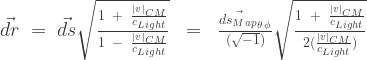

![\vec{dr}\;=\;\frac{\vec{ds}\;\;+\;\;(\frac{1}{\sqrt{-1}})[\sqrt{\frac{1 \;\;-\;\;\frac{|v|_{CM}}{c_{Light}}}{2(\frac{c_{Light}}{|v|_{CM}})}}]\,\vec{ds_{Map}}_{\theta \, \phi}}{\sqrt{1 \;\;-\;\;\frac{|v|^2_{CM}}{c^2_{Light}}}}\;=\;\frac{\vec{ds}\;\;+\;\;\vec{c_{Light}}\,[\sqrt{\frac{1 \;\;-\;\;\frac{|v|_{CM}}{c_{Light}}}{2(\frac{c_{Light}}{|v|_{CM}})}}]\,{dt_{Map}}}{\sqrt{1 \;\;-\;\;\frac{|v|^2_{CM}}{c^2_{Light}}}}](https://s0.wp.com/latex.php?latex=%5Cvec%7Bdr%7D%5C%3B%3D%5C%3B%5Cfrac%7B%5Cvec%7Bds%7D%5C%3B%5C%3B%2B%5C%3B%5C%3B%28%5Cfrac%7B1%7D%7B%5Csqrt%7B-1%7D%7D%29%5B%5Csqrt%7B%5Cfrac%7B1+%5C%3B%5C%3B-%5C%3B%5C%3B%5Cfrac%7B%7Cv%7C_%7BCM%7D%7D%7Bc_%7BLight%7D%7D%7D%7B2%28%5Cfrac%7Bc_%7BLight%7D%7D%7B%7Cv%7C_%7BCM%7D%7D%29%7D%7D%5D%5C%2C%5Cvec%7Bds_%7BMap%7D%7D_%7B%5Ctheta+%5C%2C+%5Cphi%7D%7D%7B%5Csqrt%7B1+%5C%3B%5C%3B-%5C%3B%5C%3B%5Cfrac%7B%7Cv%7C%5E2_%7BCM%7D%7D%7Bc%5E2_%7BLight%7D%7D%7D%7D%5C%3B%3D%5C%3B%5Cfrac%7B%5Cvec%7Bds%7D%5C%3B%5C%3B%2B%5C%3B%5C%3B%5Cvec%7Bc_%7BLight%7D%7D%5C%2C%5B%5Csqrt%7B%5Cfrac%7B1+%5C%3B%5C%3B-%5C%3B%5C%3B%5Cfrac%7B%7Cv%7C_%7BCM%7D%7D%7Bc_%7BLight%7D%7D%7D%7B2%28%5Cfrac%7Bc_%7BLight%7D%7D%7B%7Cv%7C_%7BCM%7D%7D%29%7D%7D%5D%5C%2C%7Bdt_%7BMap%7D%7D%7D%7B%5Csqrt%7B1+%5C%3B%5C%3B-%5C%3B%5C%3B%5Cfrac%7B%7Cv%7C%5E2_%7BCM%7D%7D%7Bc%5E2_%7BLight%7D%7D%7D%7D&bg=ffffff&fg=333333&s=1&c=20201002)


 ) – measured in the
  ), relative to the
  ), relative to the

![{dt_{Light}}\;=\;\;\frac{{dt'_{Light(s)}}\;\;+\;\;[\sqrt{\frac{1 \;\;-\;\;\frac{|v|_{CM}}{c_{Light}}}{2(\frac{c_{Light}}{|v|_{CM}})}}]\,{dt_{Map}}}{\sqrt{1\;\;-\;\;\frac{|v|^2_{CM}}{c^2_{Light}}}}\;=\;\frac{{dt'_{Light(s)}}\;\;+\;\;(\frac{1}{\sqrt{-1}})(\frac{1}{{c_{Light}}})[\sqrt{\frac{1 \;\;-\;\;\frac{|v|_{CM}}{c_{Light}}}{2(\frac{c_{Light}}{|v|_{CM}})}}]\,\vec{ds_{Map}}_{\theta \, \phi}}{\sqrt{1 \;\;-\;\;\frac{|v|^2_{CM}}{c^2_{Light}}}}](https://s0.wp.com/latex.php?latex=%7Bdt_%7BLight%7D%7D%5C%3B%3D%5C%3B%5C%3B%5Cfrac%7B%7Bdt%27_%7BLight%28s%29%7D%7D%5C%3B%5C%3B%2B%5C%3B%5C%3B%5B%5Csqrt%7B%5Cfrac%7B1+%5C%3B%5C%3B-%5C%3B%5C%3B%5Cfrac%7B%7Cv%7C_%7BCM%7D%7D%7Bc_%7BLight%7D%7D%7D%7B2%28%5Cfrac%7Bc_%7BLight%7D%7D%7B%7Cv%7C_%7BCM%7D%7D%29%7D%7D%5D%5C%2C%7Bdt_%7BMap%7D%7D%7D%7B%5Csqrt%7B1%5C%3B%5C%3B-%5C%3B%5C%3B%5Cfrac%7B%7Cv%7C%5E2_%7BCM%7D%7D%7Bc%5E2_%7BLight%7D%7D%7D%7D%5C%3B%3D%5C%3B%5Cfrac%7B%7Bdt%27_%7BLight%28s%29%7D%7D%5C%3B%5C%3B%2B%5C%3B%5C%3B%28%5Cfrac%7B1%7D%7B%5Csqrt%7B-1%7D%7D%29%28%5Cfrac%7B1%7D%7B%7Bc_%7BLight%7D%7D%7D%29%5B%5Csqrt%7B%5Cfrac%7B1+%5C%3B%5C%3B-%5C%3B%5C%3B%5Cfrac%7B%7Cv%7C_%7BCM%7D%7D%7Bc_%7BLight%7D%7D%7D%7B2%28%5Cfrac%7Bc_%7BLight%7D%7D%7B%7Cv%7C_%7BCM%7D%7D%29%7D%7D%5D%5C%2C%5Cvec%7Bds_%7BMap%7D%7D_%7B%5Ctheta+%5C%2C+%5Cphi%7D%7D%7B%5Csqrt%7B1+%5C%3B%5C%3B-%5C%3B%5C%3B%5Cfrac%7B%7Cv%7C%5E2_%7BCM%7D%7D%7Bc%5E2_%7BLight%7D%7D%7D%7D&bg=ffffff&fg=333333&s=1&c=20201002)
 ) Coordinate Axes
![\vec{ds}\; = \; \begin{bmatrix} \vec{d{r}} \\[0.3em] \vec{ds_{Map}}_{\theta \, \phi} \end{bmatrix}\;= \; \begin{bmatrix} \vec{d{r}} \\[0.3em] \vec{d{r}}_{\theta} \\[0.3em] \vec{d{r}}_{\phi} \end{bmatrix} =\; \begin{bmatrix} {d{r}}\,\hat{a}_{r} \\[0.3em] {d{r}}_{\theta}\,\hat{a}_{\theta} \\[0.3em] {d{r}}_{\phi}\,\hat{a}_{\phi} \end{bmatrix} = \; \begin{bmatrix} dr\,\hat{a}_{r} \\[0.3em] {r}\;d\theta_{Lat}\,\hat{a}_{\theta} \\[0.3em] {r}\,sin\theta_{Lat}\,d\phi_{Lon}\,\hat{a}_{\phi} \end{bmatrix}\;](https://s0.wp.com/latex.php?latex=%5Cvec%7Bds%7D%5C%3B+%3D+%5C%3B+%5Cbegin%7Bbmatrix%7D+%5Cvec%7Bd%7Br%7D%7D+%5C%5C%5B0.3em%5D+%5Cvec%7Bds_%7BMap%7D%7D_%7B%5Ctheta+%5C%2C+%5Cphi%7D+%5Cend%7Bbmatrix%7D%5C%3B%3D+%5C%3B+%5Cbegin%7Bbmatrix%7D+%5Cvec%7Bd%7Br%7D%7D+%5C%5C%5B0.3em%5D+%5Cvec%7Bd%7Br%7D%7D_%7B%5Ctheta%7D+%5C%5C%5B0.3em%5D+%5Cvec%7Bd%7Br%7D%7D_%7B%5Cphi%7D+%5Cend%7Bbmatrix%7D+%3D%5C%3B+%5Cbegin%7Bbmatrix%7D+%7Bd%7Br%7D%7D%5C%2C%5Chat%7Ba%7D_%7Br%7D+%5C%5C%5B0.3em%5D+%7Bd%7Br%7D%7D_%7B%5Ctheta%7D%5C%2C%5Chat%7Ba%7D_%7B%5Ctheta%7D+%5C%5C%5B0.3em%5D+%7Bd%7Br%7D%7D_%7B%5Cphi%7D%5C%2C%5Chat%7Ba%7D_%7B%5Cphi%7D+%5Cend%7Bbmatrix%7D+%3D+%5C%3B+%5Cbegin%7Bbmatrix%7D+dr%5C%2C%5Chat%7Ba%7D_%7Br%7D+%5C%5C%5B0.3em%5D+%7Br%7D%5C%3Bd%5Ctheta_%7BLat%7D%5C%2C%5Chat%7Ba%7D_%7B%5Ctheta%7D+%5C%5C%5B0.3em%5D+%7Br%7D%5C%2Csin%5Ctheta_%7BLat%7D%5C%2Cd%5Cphi_%7BLon%7D%5C%2C%5Chat%7Ba%7D_%7B%5Cphi%7D+%5Cend%7Bbmatrix%7D%5C%3B&bg=ffffff&fg=333333&s=1&c=20201002)
![\vec{ds}\;=\;{ds}\,\hat{a}_{r}\;=\;\begin{bmatrix} [(sin\theta_{Lat}\,cos\phi_{Lon})\,\hat{a}_{x} \; +\;(\,sin\theta_{Lat}\,sin\phi_{Lon})\,\hat{a}_{y}\; +\;(cos\theta_{Lat})\,\hat{a}_{z}]{dr} \\[0.3em] [(cos\theta_{Lat}\,cos\phi_{Lon})\,\hat{a}_{x} \;+\;(\,cos\theta_{Lat}\,sin\phi_{Lon})\,\hat{a}_{y}\; -\;(sin\theta_{Lat})\,\hat{a}_{z}]\,{d{r}}_{\theta}\\[0.3em] [(sin\phi_{Lon})\,\hat{a}_{x} \;\;\; +\;\;\;(cos\phi_{Lon})\,\hat{a}_{y}\;\;\; +\;\;\;(0)\,\hat{a}_{z})]\,{d{r}}_{\phi} \end{bmatrix}\;](https://s0.wp.com/latex.php?latex=%5Cvec%7Bds%7D%5C%3B%3D%5C%3B%7Bds%7D%5C%2C%5Chat%7Ba%7D_%7Br%7D%5C%3B%3D%5C%3B%5Cbegin%7Bbmatrix%7D+%5B%28sin%5Ctheta_%7BLat%7D%5C%2Ccos%5Cphi_%7BLon%7D%29%5C%2C%5Chat%7Ba%7D_%7Bx%7D+%5C%3B+%2B%5C%3B%28%5C%2Csin%5Ctheta_%7BLat%7D%5C%2Csin%5Cphi_%7BLon%7D%29%5C%2C%5Chat%7Ba%7D_%7By%7D%5C%3B+%2B%5C%3B%28cos%5Ctheta_%7BLat%7D%29%5C%2C%5Chat%7Ba%7D_%7Bz%7D%5D%7Bdr%7D+%5C%5C%5B0.3em%5D+%5B%28cos%5Ctheta_%7BLat%7D%5C%2Ccos%5Cphi_%7BLon%7D%29%5C%2C%5Chat%7Ba%7D_%7Bx%7D+%5C%3B%2B%5C%3B%28%5C%2Ccos%5Ctheta_%7BLat%7D%5C%2Csin%5Cphi_%7BLon%7D%29%5C%2C%5Chat%7Ba%7D_%7By%7D%5C%3B+-%5C%3B%28sin%5Ctheta_%7BLat%7D%29%5C%2C%5Chat%7Ba%7D_%7Bz%7D%5D%5C%2C%7Bd%7Br%7D%7D_%7B%5Ctheta%7D%5C%5C%5B0.3em%5D+%5B%28sin%5Cphi_%7BLon%7D%29%5C%2C%5Chat%7Ba%7D_%7Bx%7D+%5C%3B%5C%3B%5C%3B+%2B%5C%3B%5C%3B%5C%3B%28cos%5Cphi_%7BLon%7D%29%5C%2C%5Chat%7Ba%7D_%7By%7D%5C%3B%5C%3B%5C%3B+%2B%5C%3B%5C%3B%5C%3B%280%29%5C%2C%5Chat%7Ba%7D_%7Bz%7D%29%5D%5C%2C%7Bd%7Br%7D%7D_%7B%5Cphi%7D+%5Cend%7Bbmatrix%7D%5C%3B&bg=ffffff&fg=333333&s=1&c=20201002)
![\vec{ds}\;=\;\vec{c_{Light}}\,{dt'_{Light(s)}}\;=\;\begin{bmatrix} \vec{dx_{s}} \\[0.3em] \vec{dy_{s}} \\[0.3em] \vec{dz_{s}} \end{bmatrix}\; = \begin{bmatrix} ds(sin\theta_{Lat}\,cos\phi_{Lon})\,\hat{a}_{x} \\[0.3em] ds(sin\theta_{Lat}\,sin\phi_{Lon})\,\hat{a}_{y} \\[0.3em] ds(cos\theta_{Lat})\,\hat{a}_{z} \end{bmatrix}\;](https://s0.wp.com/latex.php?latex=%5Cvec%7Bds%7D%5C%3B%3D%5C%3B%5Cvec%7Bc_%7BLight%7D%7D%5C%2C%7Bdt%27_%7BLight%28s%29%7D%7D%5C%3B%3D%5C%3B%5Cbegin%7Bbmatrix%7D+%5Cvec%7Bdx_%7Bs%7D%7D+%5C%5C%5B0.3em%5D+%5Cvec%7Bdy_%7Bs%7D%7D+%5C%5C%5B0.3em%5D+%5Cvec%7Bdz_%7Bs%7D%7D+%5Cend%7Bbmatrix%7D%5C%3B+%3D+%5Cbegin%7Bbmatrix%7D+ds%28sin%5Ctheta_%7BLat%7D%5C%2Ccos%5Cphi_%7BLon%7D%29%5C%2C%5Chat%7Ba%7D_%7Bx%7D+%5C%5C%5B0.3em%5D+ds%28sin%5Ctheta_%7BLat%7D%5C%2Csin%5Cphi_%7BLon%7D%29%5C%2C%5Chat%7Ba%7D_%7By%7D+%5C%5C%5B0.3em%5D+ds%28cos%5Ctheta_%7BLat%7D%29%5C%2C%5Chat%7Ba%7D_%7Bz%7D+%5Cend%7Bbmatrix%7D%5C%3B&bg=ffffff&fg=333333&s=1&c=20201002)
 ), and one (1) “geodesic arc-length” component, which is the “Map/Patch/Manifold” (
 ), and the Longitude Angle (
 )
)![\vec{ds}\; = \; \begin{bmatrix} \vec{d{r}} \\[0.3em] \vec{ds_{Map}}_{\theta \, \phi} \end{bmatrix}\;= \; \begin{bmatrix} \vec{d{r}} \\[0.3em] {r}\,{\vec{d\Omega_{Map}}_{(\theta \phi)}} \end{bmatrix}\; =\; \begin{bmatrix} {d{r}}\,\hat{a}_{r} \\[0.3em] r(\sqrt{(d\theta_{Lat}\,\hat{a}_{\theta})^2 + (sin\theta_{Lat}\,d\phi_{Lon}\,\hat{a}_{\phi})^2})\,\hat{a}_{r} \end{bmatrix}\;](https://s0.wp.com/latex.php?latex=%5Cvec%7Bds%7D%5C%3B+%3D+%5C%3B+%5Cbegin%7Bbmatrix%7D+%5Cvec%7Bd%7Br%7D%7D+%5C%5C%5B0.3em%5D+%5Cvec%7Bds_%7BMap%7D%7D_%7B%5Ctheta+%5C%2C+%5Cphi%7D+%5Cend%7Bbmatrix%7D%5C%3B%3D+%5C%3B+%5Cbegin%7Bbmatrix%7D+%5Cvec%7Bd%7Br%7D%7D+%5C%5C%5B0.3em%5D+%7Br%7D%5C%2C%7B%5Cvec%7Bd%5COmega_%7BMap%7D%7D_%7B%28%5Ctheta+%5Cphi%29%7D%7D+%5Cend%7Bbmatrix%7D%5C%3B+%3D%5C%3B+%5Cbegin%7Bbmatrix%7D+%7Bd%7Br%7D%7D%5C%2C%5Chat%7Ba%7D_%7Br%7D+%5C%5C%5B0.3em%5D+r%28%5Csqrt%7B%28d%5Ctheta_%7BLat%7D%5C%2C%5Chat%7Ba%7D_%7B%5Ctheta%7D%29%5E2+%2B+%28sin%5Ctheta_%7BLat%7D%5C%2Cd%5Cphi_%7BLon%7D%5C%2C%5Chat%7Ba%7D_%7B%5Cphi%7D%29%5E2%7D%29%5C%2C%5Chat%7Ba%7D_%7Br%7D+%5Cend%7Bbmatrix%7D%5C%3B&bg=ffffff&fg=333333&s=1&c=20201002)
![\vec{ds}\; = \; \begin{bmatrix} \vec{d{r}} \\[0.3em] \vec{ds_{Map}}_{\theta \, \phi} \end{bmatrix}\;= \; \begin{bmatrix} \vec{d{r}} \\[0.3em] {r}\,{\vec{d\Omega_{Map}}_{(\theta \phi)}} \end{bmatrix}\; =\; \begin{bmatrix} {d{r}}\,\hat{a}_{r} \\[0.3em] (\sqrt{-1})[\sqrt{\frac{2(\frac{|v|_{CM}}{c_{Light}})}{1 \;\;+\;\;\frac{|v|_{CM}}{c_{Light}}}}]({dr})\;\hat{a}_{r}\end{bmatrix}\;](https://s0.wp.com/latex.php?latex=%5Cvec%7Bds%7D%5C%3B+%3D+%5C%3B+%5Cbegin%7Bbmatrix%7D+%5Cvec%7Bd%7Br%7D%7D+%5C%5C%5B0.3em%5D+%5Cvec%7Bds_%7BMap%7D%7D_%7B%5Ctheta+%5C%2C+%5Cphi%7D+%5Cend%7Bbmatrix%7D%5C%3B%3D+%5C%3B+%5Cbegin%7Bbmatrix%7D+%5Cvec%7Bd%7Br%7D%7D+%5C%5C%5B0.3em%5D+%7Br%7D%5C%2C%7B%5Cvec%7Bd%5COmega_%7BMap%7D%7D_%7B%28%5Ctheta+%5Cphi%29%7D%7D+%5Cend%7Bbmatrix%7D%5C%3B+%3D%5C%3B+%5Cbegin%7Bbmatrix%7D+%7Bd%7Br%7D%7D%5C%2C%5Chat%7Ba%7D_%7Br%7D+%5C%5C%5B0.3em%5D+%28%5Csqrt%7B-1%7D%29%5B%5Csqrt%7B%5Cfrac%7B2%28%5Cfrac%7B%7Cv%7C_%7BCM%7D%7D%7Bc_%7BLight%7D%7D%29%7D%7B1+%5C%3B%5C%3B%2B%5C%3B%5C%3B%5Cfrac%7B%7Cv%7C_%7BCM%7D%7D%7Bc_%7BLight%7D%7D%7D%7D%5D%28%7Bdr%7D%29%5C%3B%5Chat%7Ba%7D_%7Br%7D%5Cend%7Bbmatrix%7D%5C%3B&bg=ffffff&fg=333333&s=1&c=20201002)
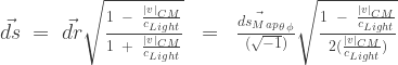

![\vec{ds}\;=\;\frac{\vec{dr}\;\;-\;\;(\frac{1}{\sqrt{-1}})[\sqrt{\frac{1 \;\;+\;\;\frac{|v|_{CM}}{c_{Light}}}{2(\frac{c_{Light}}{|v|_{CM}})}}]\,\vec{ds_{Map}}_{\theta \, \phi}}{\sqrt{1 \;\;-\;\;\frac{|v|^2_{CM}}{c^2_{Light}}}}\;=\;\frac{\vec{dr}\;\;-\;\;\vec{c_{Light}}\,[\sqrt{\frac{1 \;\;+\;\;\frac{|v|_{CM}}{c_{Light}}}{2(\frac{c_{Light}}{|v|_{CM}})}}]\,{dt_{Map}}}{\sqrt{1 \;\;-\;\;\frac{|v|^2_{CM}}{c^2_{Light}}}}](https://s0.wp.com/latex.php?latex=%5Cvec%7Bds%7D%5C%3B%3D%5C%3B%5Cfrac%7B%5Cvec%7Bdr%7D%5C%3B%5C%3B-%5C%3B%5C%3B%28%5Cfrac%7B1%7D%7B%5Csqrt%7B-1%7D%7D%29%5B%5Csqrt%7B%5Cfrac%7B1+%5C%3B%5C%3B%2B%5C%3B%5C%3B%5Cfrac%7B%7Cv%7C_%7BCM%7D%7D%7Bc_%7BLight%7D%7D%7D%7B2%28%5Cfrac%7Bc_%7BLight%7D%7D%7B%7Cv%7C_%7BCM%7D%7D%29%7D%7D%5D%5C%2C%5Cvec%7Bds_%7BMap%7D%7D_%7B%5Ctheta+%5C%2C+%5Cphi%7D%7D%7B%5Csqrt%7B1+%5C%3B%5C%3B-%5C%3B%5C%3B%5Cfrac%7B%7Cv%7C%5E2_%7BCM%7D%7D%7Bc%5E2_%7BLight%7D%7D%7D%7D%5C%3B%3D%5C%3B%5Cfrac%7B%5Cvec%7Bdr%7D%5C%3B%5C%3B-%5C%3B%5C%3B%5Cvec%7Bc_%7BLight%7D%7D%5C%2C%5B%5Csqrt%7B%5Cfrac%7B1+%5C%3B%5C%3B%2B%5C%3B%5C%3B%5Cfrac%7B%7Cv%7C_%7BCM%7D%7D%7Bc_%7BLight%7D%7D%7D%7B2%28%5Cfrac%7Bc_%7BLight%7D%7D%7B%7Cv%7C_%7BCM%7D%7D%29%7D%7D%5D%5C%2C%7Bdt_%7BMap%7D%7D%7D%7B%5Csqrt%7B1+%5C%3B%5C%3B-%5C%3B%5C%3B%5Cfrac%7B%7Cv%7C%5E2_%7BCM%7D%7D%7Bc%5E2_%7BLight%7D%7D%7D%7D&bg=ffffff&fg=333333&s=1&c=20201002)


 ) – measured in the
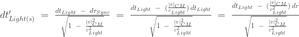
![{dt'_{Light(s)}}\;=\;\frac{\vec{dt_{Light}}\;\;-\;\;[\sqrt{\frac{1 \;\;+\;\;\frac{|v|_{CM}}{c_{Light}}}{2(\frac{c_{Light}}{|v|_{CM}})}}]\,{dt_{Map}}}{\sqrt{1 \;\;-\;\;\frac{|v|^2_{CM}}{c^2_{Light}}}}\;=\;\frac{\vec{dt_{Light}}\;\;-\;\;(\frac{1}{\sqrt{-1}})(\frac{1}{{c_{Light}}})[\sqrt{\frac{1 \;\;+\;\;\frac{|v|_{CM}}{c_{Light}}}{2(\frac{c_{Light}}{|v|_{CM}})}}]\,\vec{ds_{Map}}_{\theta \, \phi}}{\sqrt{1 \;\;-\;\;\frac{|v|^2_{CM}}{c^2_{Light}}}}](https://s0.wp.com/latex.php?latex=%7Bdt%27_%7BLight%28s%29%7D%7D%5C%3B%3D%5C%3B%5Cfrac%7B%5Cvec%7Bdt_%7BLight%7D%7D%5C%3B%5C%3B-%5C%3B%5C%3B%5B%5Csqrt%7B%5Cfrac%7B1+%5C%3B%5C%3B%2B%5C%3B%5C%3B%5Cfrac%7B%7Cv%7C_%7BCM%7D%7D%7Bc_%7BLight%7D%7D%7D%7B2%28%5Cfrac%7Bc_%7BLight%7D%7D%7B%7Cv%7C_%7BCM%7D%7D%29%7D%7D%5D%5C%2C%7Bdt_%7BMap%7D%7D%7D%7B%5Csqrt%7B1+%5C%3B%5C%3B-%5C%3B%5C%3B%5Cfrac%7B%7Cv%7C%5E2_%7BCM%7D%7D%7Bc%5E2_%7BLight%7D%7D%7D%7D%5C%3B%3D%5C%3B%5Cfrac%7B%5Cvec%7Bdt_%7BLight%7D%7D%5C%3B%5C%3B-%5C%3B%5C%3B%28%5Cfrac%7B1%7D%7B%5Csqrt%7B-1%7D%7D%29%28%5Cfrac%7B1%7D%7B%7Bc_%7BLight%7D%7D%7D%29%5B%5Csqrt%7B%5Cfrac%7B1+%5C%3B%5C%3B%2B%5C%3B%5C%3B%5Cfrac%7B%7Cv%7C_%7BCM%7D%7D%7Bc_%7BLight%7D%7D%7D%7B2%28%5Cfrac%7Bc_%7BLight%7D%7D%7B%7Cv%7C_%7BCM%7D%7D%29%7D%7D%5D%5C%2C%5Cvec%7Bds_%7BMap%7D%7D_%7B%5Ctheta+%5C%2C+%5Cphi%7D%7D%7B%5Csqrt%7B1+%5C%3B%5C%3B-%5C%3B%5C%3B%5Cfrac%7B%7Cv%7C%5E2_%7BCM%7D%7D%7Bc%5E2_%7BLight%7D%7D%7D%7D&bg=ffffff&fg=333333&s=1&c=20201002)
 ) – is a vector (direction dependent) described in Spherical (
 ) Coordinate Axes
![\vec{d\Omega_{Map}}_{(\theta \phi)}\; = {d\Omega_{Map}}_{(\theta \phi)}\,\hat{a}_{r}\; =\; \begin{bmatrix} \vec{d\theta_{Lat}} \\[0.3em] \vec{d\phi_{Lon}} \end{bmatrix}\;= \; \begin{bmatrix} d\theta_{Lat}\,\hat{a}_{\theta} \\[0.3em] sin\theta_{Lat}\,d\phi_{Lon}\,\hat{a}_{\phi} \end{bmatrix}\;](https://s0.wp.com/latex.php?latex=%5Cvec%7Bd%5COmega_%7BMap%7D%7D_%7B%28%5Ctheta+%5Cphi%29%7D%5C%3B+%3D+%7Bd%5COmega_%7BMap%7D%7D_%7B%28%5Ctheta+%5Cphi%29%7D%5C%2C%5Chat%7Ba%7D_%7Br%7D%5C%3B+%3D%5C%3B+%5Cbegin%7Bbmatrix%7D+%5Cvec%7Bd%5Ctheta_%7BLat%7D%7D+%5C%5C%5B0.3em%5D+%5Cvec%7Bd%5Cphi_%7BLon%7D%7D+%5Cend%7Bbmatrix%7D%5C%3B%3D+%5C%3B+%5Cbegin%7Bbmatrix%7D+d%5Ctheta_%7BLat%7D%5C%2C%5Chat%7Ba%7D_%7B%5Ctheta%7D+%5C%5C%5B0.3em%5D+sin%5Ctheta_%7BLat%7D%5C%2Cd%5Cphi_%7BLon%7D%5C%2C%5Chat%7Ba%7D_%7B%5Cphi%7D+%5Cend%7Bbmatrix%7D%5C%3B&bg=ffffff&fg=333333&s=1&c=20201002)

![\vec{d\Omega_{Map}}_{(\theta \phi)}\; = {d\Omega_{Map}}_{(\theta \phi)}\,\hat{a}_{r}\; = \; \begin{bmatrix}[(cos\theta_{Lat}\,cos\phi_{Lon})\,\hat{a}_{x} \;+\;(\,cos\theta_{Lat}\,sin\phi_{Lon})\,\hat{a}_{y}\; -\;(sin\theta_{Lat})\,\hat{a}_{z}]\,d{\theta}\\[0.3em] [(sin\phi_{Lon})\,\hat{a}_{x} \;\;\; +\;\;\;(cos\phi_{Lon})\,\hat{a}_{y}\;\;\; +\;\;\;(0)\,\hat{a}_{z})]\,d{\phi} \end{bmatrix}\;](https://s0.wp.com/latex.php?latex=%5Cvec%7Bd%5COmega_%7BMap%7D%7D_%7B%28%5Ctheta+%5Cphi%29%7D%5C%3B+%3D+%7Bd%5COmega_%7BMap%7D%7D_%7B%28%5Ctheta+%5Cphi%29%7D%5C%2C%5Chat%7Ba%7D_%7Br%7D%5C%3B+%3D+%5C%3B+%5Cbegin%7Bbmatrix%7D%5B%28cos%5Ctheta_%7BLat%7D%5C%2Ccos%5Cphi_%7BLon%7D%29%5C%2C%5Chat%7Ba%7D_%7Bx%7D+%5C%3B%2B%5C%3B%28%5C%2Ccos%5Ctheta_%7BLat%7D%5C%2Csin%5Cphi_%7BLon%7D%29%5C%2C%5Chat%7Ba%7D_%7By%7D%5C%3B+-%5C%3B%28sin%5Ctheta_%7BLat%7D%29%5C%2C%5Chat%7Ba%7D_%7Bz%7D%5D%5C%2Cd%7B%5Ctheta%7D%5C%5C%5B0.3em%5D+%5B%28sin%5Cphi_%7BLon%7D%29%5C%2C%5Chat%7Ba%7D_%7Bx%7D+%5C%3B%5C%3B%5C%3B+%2B%5C%3B%5C%3B%5C%3B%28cos%5Cphi_%7BLon%7D%29%5C%2C%5Chat%7Ba%7D_%7By%7D%5C%3B%5C%3B%5C%3B+%2B%5C%3B%5C%3B%5C%3B%280%29%5C%2C%5Chat%7Ba%7D_%7Bz%7D%29%5D%5C%2Cd%7B%5Cphi%7D+%5Cend%7Bbmatrix%7D%5C%3B&bg=ffffff&fg=333333&s=1&c=20201002)


\;\hat{a}_{r}\;=\;(\sqrt{-1})[\sqrt{\frac{2(\frac{|v|_{CM}}{c_{Light}})}{1 \;\;-\;\;\frac{|v|_{CM}}{c_{Light}}}}](\frac{ds}{r})\;\hat{a}_{r}](https://s0.wp.com/latex.php?latex=%5Cvec%7Bd%5COmega_%7BMap%7D%7D_%7B%28%5Ctheta+%5Cphi%29%7D%5C%3B%3D%5C%3B%28%5Csqrt%7B-1%7D%29%5B%5Csqrt%7B%5Cfrac%7B2%28%5Cfrac%7B%7Cv%7C_%7BCM%7D%7D%7Bc_%7BLight%7D%7D%29%7D%7B1+%5C%3B%5C%3B%2B%5C%3B%5C%3B%5Cfrac%7B%7Cv%7C_%7BCM%7D%7D%7Bc_%7BLight%7D%7D%7D%7D%5D%28%5Cfrac%7Bdr%7D%7Br%7D%29%5C%3B%5Chat%7Ba%7D_%7Br%7D%5C%3B%3D%5C%3B%28%5Csqrt%7B-1%7D%29%5B%5Csqrt%7B%5Cfrac%7B2%28%5Cfrac%7B%7Cv%7C_%7BCM%7D%7D%7Bc_%7BLight%7D%7D%29%7D%7B1+%5C%3B%5C%3B-%5C%3B%5C%3B%5Cfrac%7B%7Cv%7C_%7BCM%7D%7D%7Bc_%7BLight%7D%7D%7D%7D%5D%28%5Cfrac%7Bds%7D%7Br%7D%29%5C%3B%5Chat%7Ba%7D_%7Br%7D&bg=ffffff&fg=333333&s=1&c=20201002)
 ) in the
  ) in the

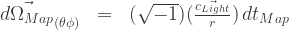


 ) – is a vector (direction dependent) described in Rectangular Cartesian (
![\vec{d\theta_{Lat}}\; = {d\theta_{Lat}}\,\hat{a}_{\theta}\; = \; \begin{bmatrix}[(cos\theta_{Lat}\,cos\phi_{Lon})\,\hat{a}_{x} \;+\;(\,cos\theta_{Lat}\,sin\phi_{Lon})\,\hat{a}_{y}\; -\;(sin\theta_{Lat})\,\hat{a}_{z}]\, d{\theta} \end{bmatrix}\;](https://s0.wp.com/latex.php?latex=%5Cvec%7Bd%5Ctheta_%7BLat%7D%7D%5C%3B+%3D+%7Bd%5Ctheta_%7BLat%7D%7D%5C%2C%5Chat%7Ba%7D_%7B%5Ctheta%7D%5C%3B+%3D+%5C%3B+%5Cbegin%7Bbmatrix%7D%5B%28cos%5Ctheta_%7BLat%7D%5C%2Ccos%5Cphi_%7BLon%7D%29%5C%2C%5Chat%7Ba%7D_%7Bx%7D+%5C%3B%2B%5C%3B%28%5C%2Ccos%5Ctheta_%7BLat%7D%5C%2Csin%5Cphi_%7BLon%7D%29%5C%2C%5Chat%7Ba%7D_%7By%7D%5C%3B+-%5C%3B%28sin%5Ctheta_%7BLat%7D%29%5C%2C%5Chat%7Ba%7D_%7Bz%7D%5D%5C%2C+d%7B%5Ctheta%7D+%5Cend%7Bbmatrix%7D%5C%3B&bg=ffffff&fg=333333&s=1&c=20201002)


 ) in the
 ) – is a vector (direction dependent) described in Rectangular Cartesian (
![\vec{d\phi_{Lon}}\; = \;{ d\phi_{Lon}}\,\hat{a}_{\phi}\; = \; \begin{bmatrix} [(sin\phi_{Lon})\,\hat{a}_{x} \;\;\; +\;\;\;(cos\phi_{Lon})\,\hat{a}_{y}\;\;\; +\;\;\;(0)\,\hat{a}_{z})]\,d{\phi} \end{bmatrix}\;](https://s0.wp.com/latex.php?latex=%5Cvec%7Bd%5Cphi_%7BLon%7D%7D%5C%3B+%3D+%5C%3B%7B+d%5Cphi_%7BLon%7D%7D%5C%2C%5Chat%7Ba%7D_%7B%5Cphi%7D%5C%3B+%3D+%5C%3B+%5Cbegin%7Bbmatrix%7D+%5B%28sin%5Cphi_%7BLon%7D%29%5C%2C%5Chat%7Ba%7D_%7Bx%7D+%5C%3B%5C%3B%5C%3B+%2B%5C%3B%5C%3B%5C%3B%28cos%5Cphi_%7BLon%7D%29%5C%2C%5Chat%7Ba%7D_%7By%7D%5C%3B%5C%3B%5C%3B+%2B%5C%3B%5C%3B%5C%3B%280%29%5C%2C%5Chat%7Ba%7D_%7Bz%7D%29%5D%5C%2Cd%7B%5Cphi%7D+%5Cend%7Bbmatrix%7D%5C%3B&bg=ffffff&fg=333333&s=1&c=20201002)

 ) in the
  ) in the
![\vec{ds_{Map}}_{\theta \, \phi}\;=\;(\sqrt{-1})\,\vec{c_{Light}}\,{dt_{Map}}\;= \; \begin{bmatrix} \vec{d{r}}_{\theta} \\[0.3em] \vec{d{r}}_{\phi} \end{bmatrix}\;= \; {r}\begin{bmatrix} d\theta_{Lat}\,\hat{a}_{\theta} \\[0.3em] sin\theta_{Lat}\,d\phi_{Lon}\,\hat{a}_{\phi} \end{bmatrix}\;](https://s0.wp.com/latex.php?latex=%5Cvec%7Bds_%7BMap%7D%7D_%7B%5Ctheta+%5C%2C+%5Cphi%7D%5C%3B%3D%5C%3B%28%5Csqrt%7B-1%7D%29%5C%2C%5Cvec%7Bc_%7BLight%7D%7D%5C%2C%7Bdt_%7BMap%7D%7D%5C%3B%3D+%5C%3B+%5Cbegin%7Bbmatrix%7D+%5Cvec%7Bd%7Br%7D%7D_%7B%5Ctheta%7D+%5C%5C%5B0.3em%5D+%5Cvec%7Bd%7Br%7D%7D_%7B%5Cphi%7D+%5Cend%7Bbmatrix%7D%5C%3B%3D+%5C%3B+%7Br%7D%5Cbegin%7Bbmatrix%7D+d%5Ctheta_%7BLat%7D%5C%2C%5Chat%7Ba%7D_%7B%5Ctheta%7D+%5C%5C%5B0.3em%5D+sin%5Ctheta_%7BLat%7D%5C%2Cd%5Cphi_%7BLon%7D%5C%2C%5Chat%7Ba%7D_%7B%5Cphi%7D+%5Cend%7Bbmatrix%7D%5C%3B&bg=ffffff&fg=333333&s=1&c=20201002)
![\vec{ds_{Map}}_{\theta \, \phi}\;=\;{ds_{Map}}_{\theta \, \phi}\,\hat{a}_{r}\;=\;\begin{bmatrix}[(cos\theta_{Lat}\,cos\phi_{Lon})\,\hat{a}_{x} \;+\;(\,cos\theta_{Lat}\,sin\phi_{Lon})\,\hat{a}_{y}\; -\;(sin\theta_{Lat})\,\hat{a}_{z}]\,{d{r}}_{\theta}\\[0.3em] [(sin\phi_{Lon})\,\hat{a}_{x} \;\;\; +\;\;\;(cos\phi_{Lon})\,\hat{a}_{y}\;\;\; +\;\;\;(0)\,\hat{a}_{z})]\,{d{r}}_{\phi} \end{bmatrix}\;](https://s0.wp.com/latex.php?latex=%5Cvec%7Bds_%7BMap%7D%7D_%7B%5Ctheta+%5C%2C+%5Cphi%7D%5C%3B%3D%5C%3B%7Bds_%7BMap%7D%7D_%7B%5Ctheta+%5C%2C+%5Cphi%7D%5C%2C%5Chat%7Ba%7D_%7Br%7D%5C%3B%3D%5C%3B%5Cbegin%7Bbmatrix%7D%5B%28cos%5Ctheta_%7BLat%7D%5C%2Ccos%5Cphi_%7BLon%7D%29%5C%2C%5Chat%7Ba%7D_%7Bx%7D+%5C%3B%2B%5C%3B%28%5C%2Ccos%5Ctheta_%7BLat%7D%5C%2Csin%5Cphi_%7BLon%7D%29%5C%2C%5Chat%7Ba%7D_%7By%7D%5C%3B+-%5C%3B%28sin%5Ctheta_%7BLat%7D%29%5C%2C%5Chat%7Ba%7D_%7Bz%7D%5D%5C%2C%7Bd%7Br%7D%7D_%7B%5Ctheta%7D%5C%5C%5B0.3em%5D+%5B%28sin%5Cphi_%7BLon%7D%29%5C%2C%5Chat%7Ba%7D_%7Bx%7D+%5C%3B%5C%3B%5C%3B+%2B%5C%3B%5C%3B%5C%3B%28cos%5Cphi_%7BLon%7D%29%5C%2C%5Chat%7Ba%7D_%7By%7D%5C%3B%5C%3B%5C%3B+%2B%5C%3B%5C%3B%5C%3B%280%29%5C%2C%5Chat%7Ba%7D_%7Bz%7D%29%5D%5C%2C%7Bd%7Br%7D%7D_%7B%5Cphi%7D+%5Cend%7Bbmatrix%7D%5C%3B&bg=ffffff&fg=333333&s=1&c=20201002)
 ) Coordinates mixed with Rectangular Cartesian (
 ) Coordinates, and directed along the Rectangular (
![\vec{ds_{Map}}_{\theta \, \phi}\;=\;(\sqrt{-1})\,\vec{c_{Light}}\,{dt_{Map}}\;=\;\begin{bmatrix} \vec{dx_{Map}} \\[0.3em] \vec{dy_{Map}} \\[0.3em] \vec{dz_{Map}} \end{bmatrix}\; = \begin{bmatrix} {ds_{Map}}_{\theta \, \phi}(sin\theta_{Lat}\,cos\phi_{Lon})\,\hat{a}_{x} \\[0.3em] {ds_{Map}}_{\theta \, \phi}(sin\theta_{Lat}\,sin\phi_{Lon})\,\hat{a}_{y} \\[0.3em] {ds_{Map}}_{\theta \, \phi}(cos\theta_{Lat})\,\hat{a}_{z} \end{bmatrix}\;](https://s0.wp.com/latex.php?latex=%5Cvec%7Bds_%7BMap%7D%7D_%7B%5Ctheta+%5C%2C+%5Cphi%7D%5C%3B%3D%5C%3B%28%5Csqrt%7B-1%7D%29%5C%2C%5Cvec%7Bc_%7BLight%7D%7D%5C%2C%7Bdt_%7BMap%7D%7D%5C%3B%3D%5C%3B%5Cbegin%7Bbmatrix%7D+%5Cvec%7Bdx_%7BMap%7D%7D+%5C%5C%5B0.3em%5D+%5Cvec%7Bdy_%7BMap%7D%7D+%5C%5C%5B0.3em%5D+%5Cvec%7Bdz_%7BMap%7D%7D+%5Cend%7Bbmatrix%7D%5C%3B+%3D+%5Cbegin%7Bbmatrix%7D+%7Bds_%7BMap%7D%7D_%7B%5Ctheta+%5C%2C+%5Cphi%7D%28sin%5Ctheta_%7BLat%7D%5C%2Ccos%5Cphi_%7BLon%7D%29%5C%2C%5Chat%7Ba%7D_%7Bx%7D+%5C%5C%5B0.3em%5D+%7Bds_%7BMap%7D%7D_%7B%5Ctheta+%5C%2C+%5Cphi%7D%28sin%5Ctheta_%7BLat%7D%5C%2Csin%5Cphi_%7BLon%7D%29%5C%2C%5Chat%7Ba%7D_%7By%7D+%5C%5C%5B0.3em%5D+%7Bds_%7BMap%7D%7D_%7B%5Ctheta+%5C%2C+%5Cphi%7D%28cos%5Ctheta_%7BLat%7D%29%5C%2C%5Chat%7Ba%7D_%7Bz%7D+%5Cend%7Bbmatrix%7D%5C%3B&bg=ffffff&fg=333333&s=1&c=20201002)


\;\hat{a}_{r}\;=\;(\sqrt{-1})[\sqrt{\frac{2(\frac{|v|_{CM}}{c_{Light}})}{1\;\;-\;\;\frac{|v|_{CM}}{c_{Light}}}}]({ds})\;\hat{a}_{r}](https://s0.wp.com/latex.php?latex=%5Cvec%7Bds_%7BMap%7D%7D_%7B%5Ctheta+%5C%2C+%5Cphi%7D%5C%3B%3D%5C%3B%28%5Csqrt%7B-1%7D%29%5B%5Csqrt%7B%5Cfrac%7B2%28%5Cfrac%7B%7Cv%7C_%7BCM%7D%7D%7Bc_%7BLight%7D%7D%29%7D%7B1+%5C%3B%5C%3B%2B%5C%3B%5C%3B%5Cfrac%7B%7Cv%7C_%7BCM%7D%7D%7Bc_%7BLight%7D%7D%7D%7D%5D%28%7Bdr%7D%29%5C%3B%5Chat%7Ba%7D_%7Br%7D%5C%3B%3D%5C%3B%28%5Csqrt%7B-1%7D%29%5B%5Csqrt%7B%5Cfrac%7B2%28%5Cfrac%7B%7Cv%7C_%7BCM%7D%7D%7Bc_%7BLight%7D%7D%29%7D%7B1%5C%3B%5C%3B-%5C%3B%5C%3B%5Cfrac%7B%7Cv%7C_%7BCM%7D%7D%7Bc_%7BLight%7D%7D%7D%7D%5D%28%7Bds%7D%29%5C%3B%5Chat%7Ba%7D_%7Br%7D&bg=ffffff&fg=333333&s=1&c=20201002)

 ) – measured in the


 ), and relative to the
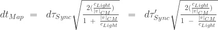

 ) for a specific potential in the gradient field is, isotropic, homogeneous, and invariant to all observers, and frames of reference, as demonstrated mathematically below.
 ) – function of Map/Patch/Manifold – “Geodesic” (
 Space & Time
![{g_{Aether}}\;\;=\;\;(\sqrt{-1})({c^2_{Light}})[\sqrt{\frac{1 \;\;+\;\;\frac{|v|_{CM}}{c_{Light}}}{2(\frac{|v|_{CM}}{c_{Light}})}}]\,\frac{\vec{d\Omega_{Map}}_{(\theta \phi)}}{\vec{dr}}\;\;=\;\;(\sqrt{-1})(\vec{c_{Light}})[\sqrt{\frac{1 \;\;+\;\;\frac{|v|_{CM}}{c_{Light}}}{2(\frac{|v|_{CM}}{c_{Light}})}}]\,\frac{\vec{d\Omega_{Map}}_{(\theta \phi)}}{{dt_{Light}}}](https://s0.wp.com/latex.php?latex=%7Bg_%7BAether%7D%7D%5C%3B%5C%3B%3D%5C%3B%5C%3B%28%5Csqrt%7B-1%7D%29%28%7Bc%5E2_%7BLight%7D%7D%29%5B%5Csqrt%7B%5Cfrac%7B1+%5C%3B%5C%3B%2B%5C%3B%5C%3B%5Cfrac%7B%7Cv%7C_%7BCM%7D%7D%7Bc_%7BLight%7D%7D%7D%7B2%28%5Cfrac%7B%7Cv%7C_%7BCM%7D%7D%7Bc_%7BLight%7D%7D%29%7D%7D%5D%5C%2C%5Cfrac%7B%5Cvec%7Bd%5COmega_%7BMap%7D%7D_%7B%28%5Ctheta+%5Cphi%29%7D%7D%7B%5Cvec%7Bdr%7D%7D%5C%3B%5C%3B%3D%5C%3B%5C%3B%28%5Csqrt%7B-1%7D%29%28%5Cvec%7Bc_%7BLight%7D%7D%29%5B%5Csqrt%7B%5Cfrac%7B1+%5C%3B%5C%3B%2B%5C%3B%5C%3B%5Cfrac%7B%7Cv%7C_%7BCM%7D%7D%7Bc_%7BLight%7D%7D%7D%7B2%28%5Cfrac%7B%7Cv%7C_%7BCM%7D%7D%7Bc_%7BLight%7D%7D%29%7D%7D%5D%5C%2C%5Cfrac%7B%5Cvec%7Bd%5COmega_%7BMap%7D%7D_%7B%28%5Ctheta+%5Cphi%29%7D%7D%7B%7Bdt_%7BLight%7D%7D%7D&bg=ffffff&fg=333333&s=1&c=20201002)
![{g_{Aether}}\;\;=\;\;(\sqrt{-1})({c^2_{Light}})[\sqrt{\frac{1 \;\;-\;\;\frac{|v|_{CM}}{c_{Light}}}{2(\frac{|v|_{CM}}{c_{Light}})}}]\,\frac{\vec{d\Omega_{Map}}_{(\theta \phi)}}{\vec{ds}}\;\;=\;\;(\sqrt{-1})(\vec{c_{Light}})[\sqrt{\frac{1 \;\;-\;\;\frac{|v|_{CM}}{c_{Light}}}{2(\frac{|v|_{CM}}{c_{Light}})}}]\,\frac{\vec{d\Omega_{Map}}_{(\theta \phi)}}{{dt'_{Light(s)}}}](https://s0.wp.com/latex.php?latex=%7Bg_%7BAether%7D%7D%5C%3B%5C%3B%3D%5C%3B%5C%3B%28%5Csqrt%7B-1%7D%29%28%7Bc%5E2_%7BLight%7D%7D%29%5B%5Csqrt%7B%5Cfrac%7B1+%5C%3B%5C%3B-%5C%3B%5C%3B%5Cfrac%7B%7Cv%7C_%7BCM%7D%7D%7Bc_%7BLight%7D%7D%7D%7B2%28%5Cfrac%7B%7Cv%7C_%7BCM%7D%7D%7Bc_%7BLight%7D%7D%29%7D%7D%5D%5C%2C%5Cfrac%7B%5Cvec%7Bd%5COmega_%7BMap%7D%7D_%7B%28%5Ctheta+%5Cphi%29%7D%7D%7B%5Cvec%7Bds%7D%7D%5C%3B%5C%3B%3D%5C%3B%5C%3B%28%5Csqrt%7B-1%7D%29%28%5Cvec%7Bc_%7BLight%7D%7D%29%5B%5Csqrt%7B%5Cfrac%7B1+%5C%3B%5C%3B-%5C%3B%5C%3B%5Cfrac%7B%7Cv%7C_%7BCM%7D%7D%7Bc_%7BLight%7D%7D%7D%7B2%28%5Cfrac%7B%7Cv%7C_%7BCM%7D%7D%7Bc_%7BLight%7D%7D%29%7D%7D%5D%5C%2C%5Cfrac%7B%5Cvec%7Bd%5COmega_%7BMap%7D%7D_%7B%28%5Ctheta+%5Cphi%29%7D%7D%7B%7Bdt%27_%7BLight%28s%29%7D%7D%7D&bg=ffffff&fg=333333&s=1&c=20201002)


![{r}\;\;=\;\;(\frac{2\,{m_{Net}}\,G}{c^2_{Light}})\,{e^{(\sqrt{-1})\,[\sqrt{{\theta^2_{Lat}}\;\;+\;\; \sin^2\theta_{Lat}\,{\phi^2_{Lon}}}]\sqrt{{\frac{1}{2}}(1\;\;+\;\; \frac{c_{Light}}{|\vec{v}|_{CM}})}}}](https://s0.wp.com/latex.php?latex=%7Br%7D%5C%3B%5C%3B%3D%5C%3B%5C%3B%28%5Cfrac%7B2%5C%2C%7Bm_%7BNet%7D%7D%5C%2CG%7D%7Bc%5E2_%7BLight%7D%7D%29%5C%2C%7Be%5E%7B%28%5Csqrt%7B-1%7D%29%5C%2C%5B%5Csqrt%7B%7B%5Ctheta%5E2_%7BLat%7D%7D%5C%3B%5C%3B%2B%5C%3B%5C%3B+%5Csin%5E2%5Ctheta_%7BLat%7D%5C%2C%7B%5Cphi%5E2_%7BLon%7D%7D%7D%5D%5Csqrt%7B%7B%5Cfrac%7B1%7D%7B2%7D%7D%281%5C%3B%5C%3B%2B%5C%3B%5C%3B+%5Cfrac%7Bc_%7BLight%7D%7D%7B%7C%5Cvec%7Bv%7D%7C_%7BCM%7D%7D%29%7D%7D%7D&bg=ffffff&fg=333333&s=1&c=20201002)

![{s}\,\,=\,\,{r_{Schwarzschild}}\,(\sqrt{1\;+\;{\theta^2_{Lat}}\;+\; \sin^2\theta_{Lat}\,{\phi^2_{Lon}}})\,{e^{(\sqrt{-1})\,[\sqrt{{\theta^2_{Lat}}\;\;+\;\; \sin^2\theta_{Lat}\,{\phi^2_{Lon}}}]\sqrt{{\frac{1}{2}}(1\;\;+\;\; \frac{c_{Light}}{|\vec{v}|_{CM}})}}}](https://s0.wp.com/latex.php?latex=%7Bs%7D%5C%2C%5C%2C%3D%5C%2C%5C%2C%7Br_%7BSchwarzschild%7D%7D%5C%2C%28%5Csqrt%7B1%5C%3B%2B%5C%3B%7B%5Ctheta%5E2_%7BLat%7D%7D%5C%3B%2B%5C%3B+%5Csin%5E2%5Ctheta_%7BLat%7D%5C%2C%7B%5Cphi%5E2_%7BLon%7D%7D%7D%29%5C%2C%7Be%5E%7B%28%5Csqrt%7B-1%7D%29%5C%2C%5B%5Csqrt%7B%7B%5Ctheta%5E2_%7BLat%7D%7D%5C%3B%5C%3B%2B%5C%3B%5C%3B+%5Csin%5E2%5Ctheta_%7BLat%7D%5C%2C%7B%5Cphi%5E2_%7BLon%7D%7D%7D%5D%5Csqrt%7B%7B%5Cfrac%7B1%7D%7B2%7D%7D%281%5C%3B%5C%3B%2B%5C%3B%5C%3B+%5Cfrac%7Bc_%7BLight%7D%7D%7B%7C%5Cvec%7Bv%7D%7C_%7BCM%7D%7D%29%7D%7D%7D&bg=ffffff&fg=333333&s=1&c=20201002)

![{s_{Map}}_{\theta \, \phi}\,\,=\,\,(\sqrt{-1})\,{r}\,[\frac{ln(\frac{r}{{r_{Schwarzschild}}})}{\sqrt{{\frac{1}{2}}(1\;\;+\;\; \frac{c_{Light}}{|\vec{v}|_{CM}})}}]\,\,=\,\,(\sqrt{-1})\,(\frac{{m_{Net}}\,G}{v^2_{Gravity}})\,[\frac{ln(\frac{r}{{r_{Schwarzschild}}})}{\sqrt{{\frac{1}{2}}(1\;\;+\;\; \frac{c_{Light}}{|\vec{v}|_{CM}})}}]](https://s0.wp.com/latex.php?latex=%7Bs_%7BMap%7D%7D_%7B%5Ctheta+%5C%2C+%5Cphi%7D%5C%2C%5C%2C%3D%5C%2C%5C%2C%28%5Csqrt%7B-1%7D%29%5C%2C%7Br%7D%5C%2C%5B%5Cfrac%7Bln%28%5Cfrac%7Br%7D%7B%7Br_%7BSchwarzschild%7D%7D%7D%29%7D%7B%5Csqrt%7B%7B%5Cfrac%7B1%7D%7B2%7D%7D%281%5C%3B%5C%3B%2B%5C%3B%5C%3B+%5Cfrac%7Bc_%7BLight%7D%7D%7B%7C%5Cvec%7Bv%7D%7C_%7BCM%7D%7D%29%7D%7D%5D%5C%2C%5C%2C%3D%5C%2C%5C%2C%28%5Csqrt%7B-1%7D%29%5C%2C%28%5Cfrac%7B%7Bm_%7BNet%7D%7D%5C%2CG%7D%7Bv%5E2_%7BGravity%7D%7D%29%5C%2C%5B%5Cfrac%7Bln%28%5Cfrac%7Br%7D%7B%7Br_%7BSchwarzschild%7D%7D%7D%29%7D%7B%5Csqrt%7B%7B%5Cfrac%7B1%7D%7B2%7D%7D%281%5C%3B%5C%3B%2B%5C%3B%5C%3B+%5Cfrac%7Bc_%7BLight%7D%7D%7B%7C%5Cvec%7Bv%7D%7C_%7BCM%7D%7D%29%7D%7D%5D&bg=ffffff&fg=333333&s=1&c=20201002)
![{g_{Aether}}\,\,=\,\,\frac{c^2_{Light}}{r}\,\,=\,\,(\sqrt{-1})\,(\frac{c^2_{Light}}{{s_{Map}}_{\theta \, \phi}})\,[\frac{ln(\frac{r}{{r_{Schwarzschild}}})}{\sqrt{{\frac{1}{2}}(1\;\;+\;\; \frac{c_{Light}}{|\vec{v}|_{CM}})}}]](https://s0.wp.com/latex.php?latex=%7Bg_%7BAether%7D%7D%5C%2C%5C%2C%3D%5C%2C%5C%2C%5Cfrac%7Bc%5E2_%7BLight%7D%7D%7Br%7D%5C%2C%5C%2C%3D%5C%2C%5C%2C%28%5Csqrt%7B-1%7D%29%5C%2C%28%5Cfrac%7Bc%5E2_%7BLight%7D%7D%7B%7Bs_%7BMap%7D%7D_%7B%5Ctheta+%5C%2C+%5Cphi%7D%7D%29%5C%2C%5B%5Cfrac%7Bln%28%5Cfrac%7Br%7D%7B%7Br_%7BSchwarzschild%7D%7D%7D%29%7D%7B%5Csqrt%7B%7B%5Cfrac%7B1%7D%7B2%7D%7D%281%5C%3B%5C%3B%2B%5C%3B%5C%3B+%5Cfrac%7Bc_%7BLight%7D%7D%7B%7C%5Cvec%7Bv%7D%7C_%7BCM%7D%7D%29%7D%7D%5D&bg=ffffff&fg=333333&s=1&c=20201002)


